
These HSC Biology Module 5 notes cover Heredity in the NSW Year 12 course: how living things reproduce, how cells copy their genetic material, how that material is used to build proteins, and how characteristics are inherited. Every idea is built up from the basics, with diagrams and worked examples.
Part of our HSC Biology notes. These notes follow the Biology Stage 6 Syllabus (2017) for the 2026 and 2027 HSC. The new syllabus is first examined in 2028.
The Working Scientifically skills section at the end teaches investigation design, data and evidence with Module 5 examples. The HSC Biology past-papers guide provides official papers and marking guidelines.
Key Takeaways
- Reproduction passes genetic information from parents to offspring: sexually, by joining two sex cells, or asexually, by copying one parent.
- Cells copy their genetic material before dividing. One kind of division keeps the number of chromosomes the same; another halves it and shuffles the versions of each gene.
- Each gene’s code is copied and read to build a protein, and the protein’s folded shape decides what it does.
- Predicting inheritance and comparing genetic material only works when you state your assumptions and use suitable evidence.
Heredity is the passing of characteristics from parents to offspring. Reproduction keeps a species going because it passes genetic information on. This module follows that information from whole organisms down to molecules and back out to populations.
Start here: the building blocks
Every later section uses these words.
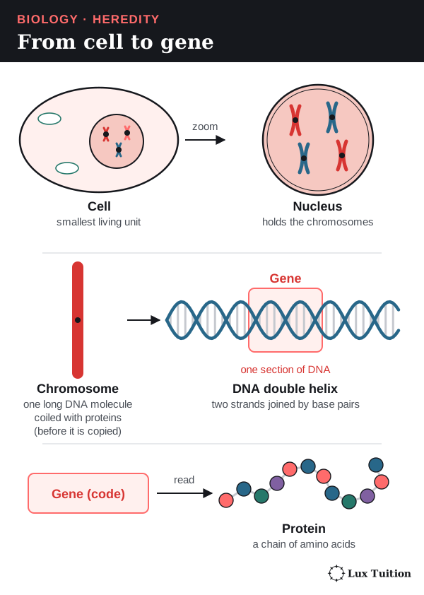
- A cell is the smallest living unit. Its cytoplasm is the jelly-like contents around the nucleus.
- The nucleus is the control centre of animal, plant and fungal cells. It holds the genetic material. Bacteria have no nucleus.
- DNA (deoxyribonucleic acid) is the molecule that stores genetic instructions. Its two long strands twist into a double helix.
- RNA (ribonucleic acid) is a single-stranded relative of DNA that helps put the instructions into action.
- A chromosome is one very long DNA molecule coiled up with proteins. Most human body cells have 46. After the DNA is copied, a chromosome has two identical DNA molecules joined together, which gives the familiar X shape.
- A gene is a section of DNA that carries the instructions for one product, usually a protein.
- An allele is one version of a gene, such as a red-petal or a white-petal version of a flower-colour gene.
- A protein is a large molecule made of a chain of amino acids (small building-block molecules; there are 20 kinds). Proteins do most of the work in cells. An enzyme is a protein that speeds up one particular reaction.
Chromosomes come in matching pairs, one from each parent.
- A diploid cell (2n) has two sets of chromosomes, one from each parent. Human body cells are diploid: 2n = 46.
- A haploid cell (n) has one set. Human sperm and eggs are haploid: n = 23.
- A gamete is a haploid sex cell, such as a sperm or an egg. Fertilisation is the joining of two gametes.
- Mitosis is cell division that keeps the chromosome number the same. Meiosis is cell division that halves it, to make haploid cells. Both are explained later.
Three ways genetic information is handled
Keep these separate; mixing them up loses marks.
- Copying: DNA replication copies a cell’s DNA.
- Rearranging: meiosis and fertilisation shuffle existing alleles into new combinations.
- Creating: a mutation is a change in the DNA sequence. Only mutation makes a brand-new allele.
How does reproduction ensure the continuity of a species?
What is the difference between sexual and asexual reproduction?
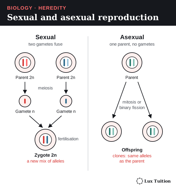
Sexual reproduction involves fertilisation: a male gamete joins a female gamete to form a zygote, the first cell of the new organism. In a typical animal, meiosis makes haploid gametes (n) and fertilisation makes a diploid zygote (2n). A self-fertilising plant makes both gametes itself, but this is still sexual reproduction.
Asexual reproduction makes offspring from one parent, without gametes fusing (no fertilisation). The offspring are usually genetically identical clones (apart from mutations). Many eukaryotes (organisms whose cells have a nucleus) reproduce asexually by mitosis. Bacteria use binary fission, which is not mitosis: bacteria have no nucleus and no spindle (the fibres that pull chromosomes apart).
Each method has a trade-off (“what happens → why it matters”):
- Asexual: fast, and no mate is needed → a successful set of alleles is copied quickly. But the clones share the same weaknesses → one new disease can harm them all.
- Sexual: new combinations of alleles → variation (differences between individuals) for natural selection to act on (better-suited individuals survive and reproduce more). But making gametes and finding mates costs energy and time.
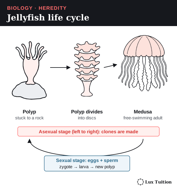
Neither method guarantees survival. Some organisms use both: strawberries reproduce sexually by flowers and asexually by runners, and many jellyfish have sexual and asexual stages.
How do internal and external fertilisation compare?
animals: advantages of external and internal fertilisation
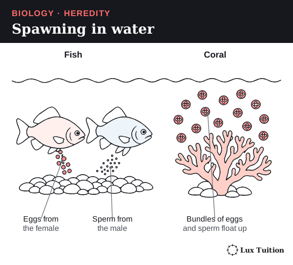
- External fertilisation happens outside the body, usually in water. Both parents release gametes and the sperm swim to the eggs.
- Internal fertilisation happens inside the female’s reproductive tract. The male places sperm close to the egg.
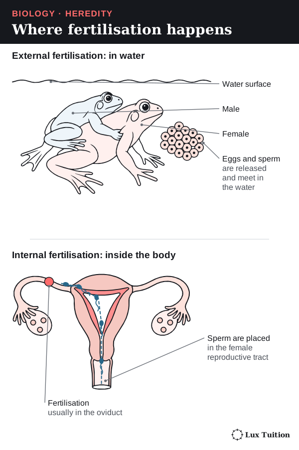
Two terms for the table below: dilution means gametes spread out in the water, so fewer sperm reach each egg; synchronised spawning means many animals release gametes into the water at the same moment.
| Feature | External fertilisation | Internal fertilisation |
|---|---|---|
| Location of gamete fusion | Outside the body, commonly in water | Within the reproductive tract |
| Mechanism and examples | Frogs can release eggs and sperm together during amplexus (the male’s mating clasp); many fish and corals release gametes into water | Sperm are transferred into the reproductive tract, bringing them close to the egg; occurs in mammals, birds and many reptiles |
| Main advantages | Many gametes can be released over an area; synchronised spawning increases encounters; substantial dispersal can occur | Gametes are protected from drying; transfer reduces dilution and can increase the chance of sperm reaching an egg |
| Main limitations | Dilution, predation and unsuitable water conditions can reduce success; timing is important | Requires successful sperm transfer; mating structures, behaviour and parental investment can carry costs |
Where does the young animal develop?
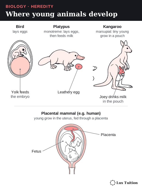
Where fertilisation happens does not decide where the embryo (the young organism growing from the zygote) develops. Birds have internal fertilisation but lay eggs.
- Oviparity: the embryo develops in a laid egg, fed mainly by yolk (a food store in the egg).
- Viviparity: live birth; how much the mother feeds the young inside her varies.
- Ovoviviparity (an older term): eggs stay inside the mother, but the embryos live mainly on yolk until they hatch.
Mammals show three patterns. Monotremes (platypus) lay eggs, then feed milk. Marsupials (kangaroos) give birth to very undeveloped young that grow on milk, often in a pouch. Placental mammals (humans) feed the fetus through a placenta, an organ joining mother and fetus. Placental young can remain dependent after birth.
Asexual reproduction in animals
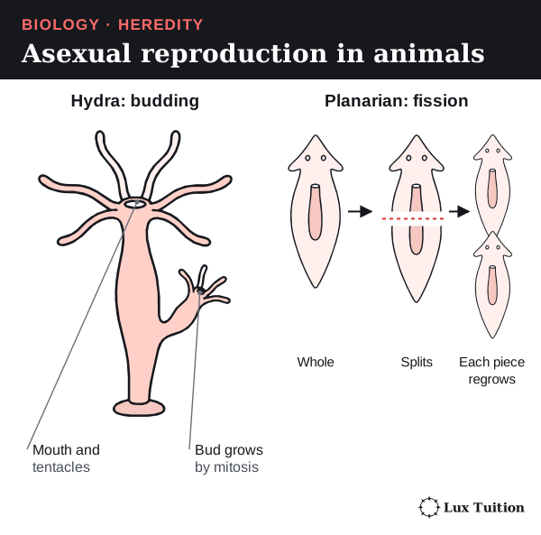
- Budding: a hydra grows a bud by mitosis, which breaks off as a new hydra.
- Fission and regeneration: some planarian flatworms split in two, and each piece regrows the missing half.
- Parthenogenesis: an embryo develops from an unfertilised egg, in some insects and some vertebrates (animals with a backbone). Genetic outcomes depend on whether and how diploidy is maintained or restored.
How do plants reproduce sexually and asexually?
plants: asexual and sexual reproduction
Asexual reproduction in plants
Vegetative propagation grows a new plant from part of a stem, root or leaf, with no flowers, seeds or gametes.
- A strawberry runner is a stem that creeps along the ground; new plants take root at points called nodes.
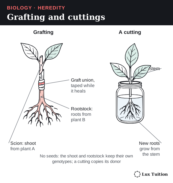
- A cutting is a piece of stem that grows adventitious roots (roots arising from a stem, sometimes helped by rooting hormones).
The new plant grows by mitosis, so it has the same genotype (set of alleles) as its parent.
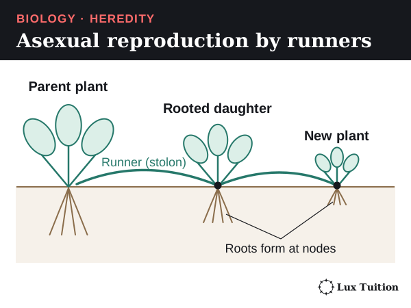
Sexual reproduction in flowering plants
A flower is the plant’s organ for sexual reproduction.
- The stamen (male part) is an anther, which makes pollen, on a stalk called a filament.
- The carpel (female part) has a sticky stigma, a stalk called the style, and an ovary holding ovules; each ovule contains an egg cell.
- Petals often attract pollinating animals; sepals protect the bud.
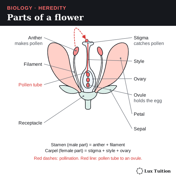
The steps, in order:
- Pollination: pollen moves from an anther to a stigma.
- A compatible pollen grain grows a pollen tube down the style to an ovule, carrying two sperm cells.
- Double fertilisation: one sperm fuses with the egg to form the diploid zygote. The other fuses with the central cell (usually two polar nuclei) to form the endosperm, usually triploid (3n), which feeds the embryo.
- The ovule becomes a seed, and the ovary usually becomes the fruit.
Pollination and fertilisation are separate events.
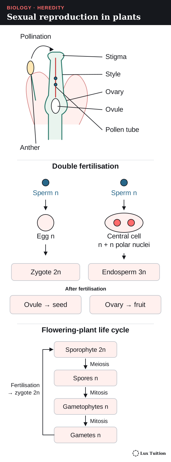
In plants, meiosis makes spores, not gametes. In the anther, meiosis makes haploid microspores, which grow by mitosis into pollen grains. So pollen is a tiny male gametophyte (gamete-making structure), not just a sperm cell. In the ovule, meiosis makes a megaspore, which grows into the female gametophyte containing the egg.
Seeds
A seed contains an embryo (the young plant), a protective seed coat that develops from maternal ovule tissues, and a food store in the endosperm and/or the cotyledons (seed leaves). These parts can have different chromosome-set numbers: the seed coat is maternal tissue, while the endosperm is usually 3n.
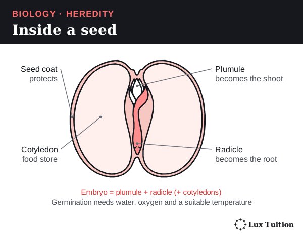
Dispersal moves seeds away from the parent. Germination restarts the embryo’s growth when it has water, oxygen and a suitable temperature. Pollination, fertilisation, dispersal and germination are separate stages.
Self-pollination and cross-pollination
- Self-pollination (pollen to a stigma of the same plant) works when pollinators are scarce, but repeated selfing increases homozygosity (two identical alleles of a gene).
- Cross-pollination (pollen to another plant) combines alleles from two plants and can increase variation.
Animal-pollinated flowers offer nectar, colour and scent; wind-pollinated plants make huge amounts of light pollen. Pollination only succeeds if the pollen is compatible and conditions are suitable.
Ferns: alternation of generations
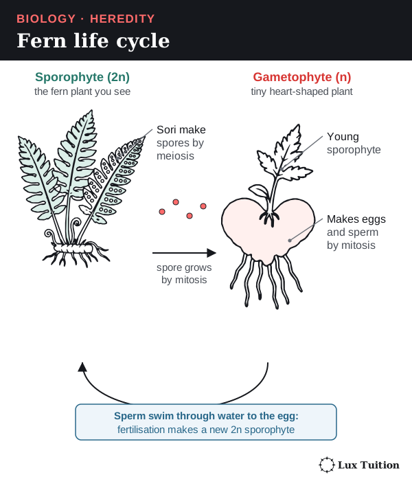
A fern’s life cycle switches between a diploid plant and a haploid plant (alternation of generations):
- The sporophyte (2n) is the leafy fern you see. It makes haploid spores by meiosis.
- A spore grows by mitosis into a small gametophyte (n).
- The gametophyte makes eggs and sperm by mitosis.
- Fertilisation makes a zygote, which grows into a new sporophyte.
So a plant spore is not a gamete, and making spores does not make the whole cycle asexual. Fern sperm must swim through water to the egg; seed plants use pollen and seeds, so they depend much less on water. Gymnosperms have unenclosed ovules and no fruits; mosses also alternate generations.
How do fungi reproduce by budding and spores?
fungi: budding, spores
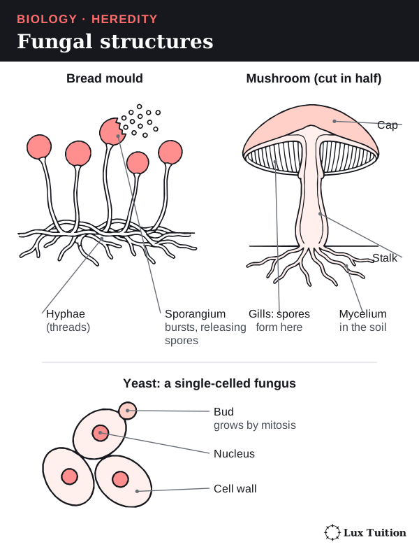
Fungi include yeasts, moulds and mushrooms. Most are made of hyphae (thin threads of cells); a mass of hyphae is a mycelium. Yeasts are single-celled.
Budding in yeast
Budding is asexual reproduction in which an outgrowth (a bud) grows from the parent and separates:
- A bud forms on the cell.
- The nucleus divides by mitosis, and one new nucleus moves into the bud.
- The bud grows, then separates.
The cytoplasm is shared unequally (the bud starts small), which distinguishes budding from splitting into two equal cells.
Spores
A spore is a reproductive cell that grows into a new organism without fusing with another cell.
- Asexual spores are made by mitosis and carry the parent’s genotype (apart from mutation); only these preserve the parental genotype.
- Sexual spores are made after meiosis and can carry new allele combinations.
Spores are tiny and numerous, so they spread far, but each still needs suitable conditions to germinate. In many fungal sexual cycles (the duration and arrangement of these stages vary among fungi):
- Plasmogamy: two compatible hyphae fuse their cytoplasm; their haploid nuclei sit side by side.
- Karyogamy: the nuclei fuse into a diploid nucleus.
- Meiosis makes haploid nuclei that end up in spores (not necessarily gametes).
Moulds make spores inside capsules called sporangia; a gilled mushroom makes basidiospores (sexual spores) on basidia (club-shaped cells) on the surface of its gills. Fragmentation is another asexual method: a broken-off piece of mycelium grows into a new fungus.
Measuring reproduction: counting cells
To show yeast is reproducing, you need evidence that cell number is increasing. A counting chamber (haemocytometer) is a microscope slide with an etched grid and a known depth, so each square holds a known volume.
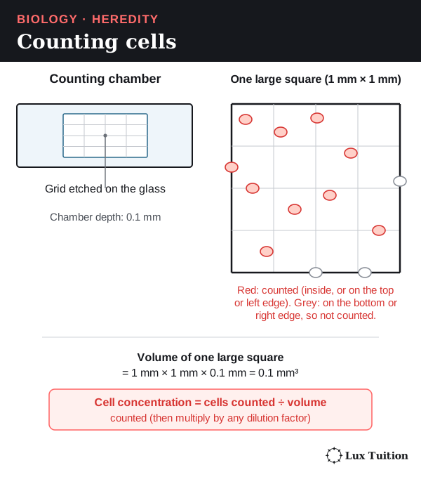
- Count the cells in a set number of squares.
- Volume counted = grid area × chamber depth.
- Cell concentration = cells counted ÷ volume counted (× any dilution factor).
- Repeat later; the change in concentration measures the net increase in cell number. Multiply by the suspension volume to estimate the total population.
A count cannot tell living cells from dead ones.
A fair temperature experiment.
The independent variable (what you change) is temperature; the dependent variable (what you measure) is the change in cell concentration over time. Controlled variables: starting concentration, volumes, nutrients and pH (how acidic or alkaline a solution is).
Sample at matched times, count squares across the whole chamber, and decide in advance the edge rule and whether an attached bud counts, so counting habits cannot look like reproduction. Independent replicate samples show real variation; recounting one sample only checks counting precision.
Risk example: yeast is low-risk, but cultures can be contaminated by other microbes (hazard) that could cause infection (harm), so use sterile technique, keep cultures covered and disinfect benches and dispose of cultures safely afterwards (precaution).
Exam trap. Carbon dioxide production shows yeast is respiring, but the amount per cell can change, so it does not directly show an increase in cell number. Saying yeast “grew” does not say what was measured either.
NESA’s 2019 Biology feedback highlights this; the known-volume principle is in Thermo Fisher’s counting-chamber reference.
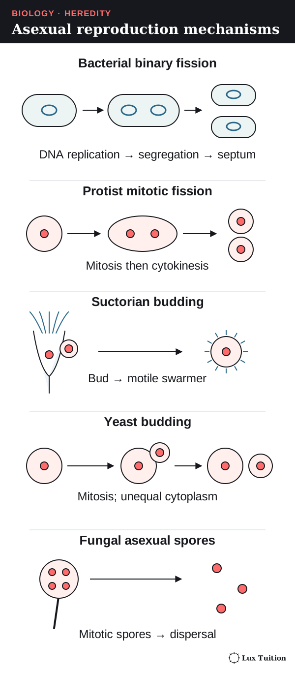
How does binary fission in bacteria compare with binary fission and budding in protists?
bacteria: binary fission (ACSBL075)
protists: binary fission, budding
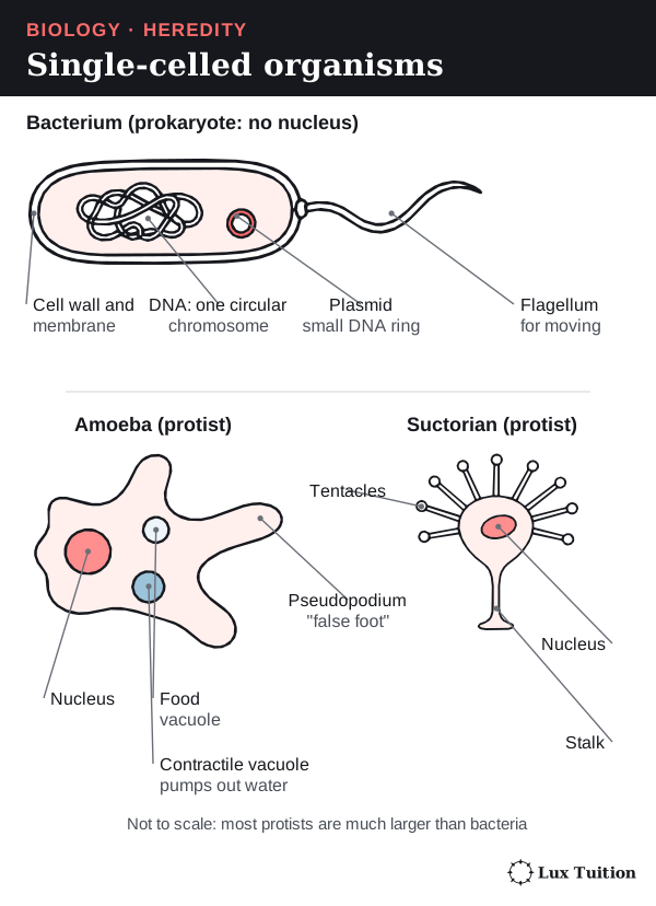
- Bacteria are single-celled prokaryotes (no nucleus). Their main DNA is usually one circular chromosome in a region called the nucleoid; many also carry plasmids (small extra rings of DNA).
- Protists, such as amoebae, are mostly single-celled eukaryotes, so their DNA is inside a nucleus.
Binary fission in bacteria
Binary fission divides one cell into two similar cells:
- DNA replication: copying of the circular chromosome starts at one point (the origin) and runs both ways round the circle.
- Chromosome segregation: the two copies move apart as the cell lengthens.
- Cell division: the membrane and cell wall (septum) form across the middle, partitioning the cytoplasm and giving two cells with one chromosome copy each.
So the order is DNA replication → chromosome segregation → cell division. There is no nuclear division, because there is no nucleus. Mutations can make daughter cells differ. Bacteria can also gain DNA by horizontal gene transfer from other bacteria, but that is not reproduction because no new cells are made.
Binary fission and budding in protists
In an amoeba’s binary fission, the nucleus divides by mitosis, then the cytoplasm divides. In multiple fission, the nucleus divides several times before the cell splits into more than two offspring.
Some protists reproduce by budding. In suctorian ciliates, an adult fixed on a stalk produces a bud covered in tiny hairs (cilia), which swims away and later becomes an adult. This is a protist example separate from yeast, which is a fungus. Ma and colleagues’ observations of suctorian ciliates.
How does the mammalian reproductive cycle produce gametes?
Mammals reproduce sexually with internal fertilisation. First the organs, then the gametes, then the hormones.
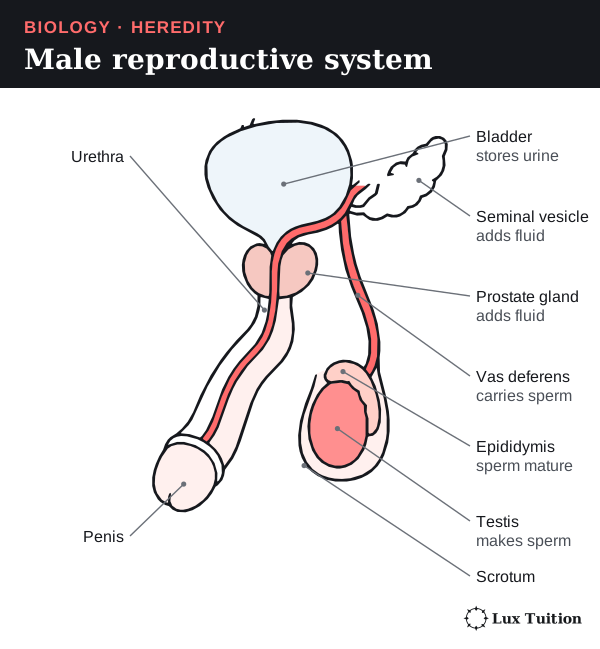
The male reproductive system
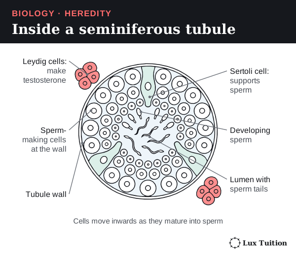
- The testes make sperm inside tiny coiled tubes called seminiferous tubules. They hang in the scrotum, which keeps them slightly cool.
- Sperm mature in the epididymis, then the vas deferens carries them to the urethra, the tube through the penis.
- The seminal vesicles and prostate gland add fluid; sperm plus fluid is semen.
The female reproductive system
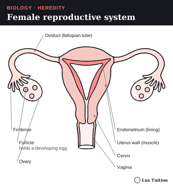
- The two ovaries hold eggs, each in a fluid-filled sac called a follicle.
- Each oviduct (fallopian tube) has finger-like fimbriae that sweep a released egg into it. Fertilisation usually happens here.
- The uterus is the muscular organ where the embryo grows. Its lining is the endometrium. Implantation is the embryo attaching to and burrowing into the endometrium.
- The cervix is the uterus’s narrow neck, opening into the vagina.
Meiosis in brief
Meiosis has two divisions, meiosis I and meiosis II. Each has four stages: prophase (chromosomes coil up), metaphase (they line up in the middle), anaphase (they are pulled apart) and telophase (new nuclei form). So prophase I is the start of the first division, and metaphase II is the line-up stage of the second. The full detail comes in the cell replication section.
Making sperm and eggs
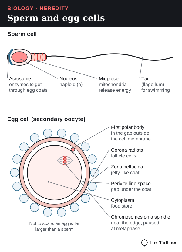
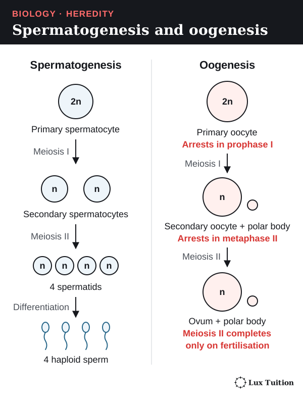
Spermatogenesis (sperm production) happens in the seminiferous tubules: a diploid cell undergoes meiosis to make four haploid cells, which each develop into a sperm. A sperm cell has:
- an acrosome with enzymes for getting through the egg’s coverings
- a nucleus with one haploid set of chromosomes
- a midpiece packed with mitochondria, which release energy as ATP (the cell’s energy-carrying molecule) for swimming
- a flagellum (tail) for swimming.
Oogenesis (egg production) also uses meiosis, with two differences:
- Unequal division: one large cell keeps most of the cytoplasm; the tiny leftover cells are polar bodies.
- Long pauses: in humans, meiosis starts before birth and primary oocytes pause at prophase I. Each cycle one primary oocyte restarts and is released at ovulation (release of an egg from the ovary) as a secondary oocyte, paused at metaphase II. It finishes meiosis II only if a sperm fertilises it.
Calling every stage an “ovum” hides these changes, so use the exact names in exams.
Hormones that control reproduction
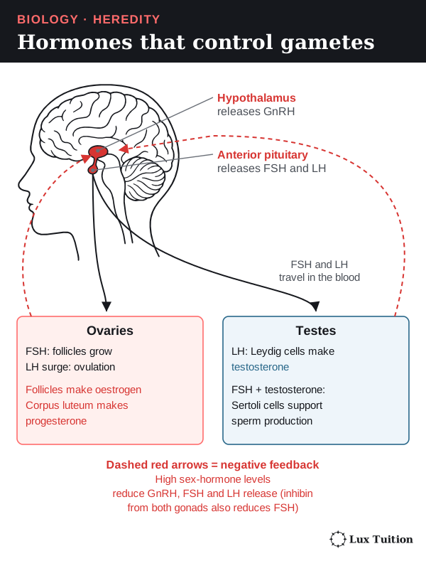
A hormone is a chemical messenger made by a gland and carried in the blood to target cells. Three glands work in a chain:
- The hypothalamus (in the brain) releases GnRH (gonadotrophin-releasing hormone).
- GnRH makes the anterior pituitary release FSH (follicle-stimulating hormone) and LH (luteinising hormone).
- FSH and LH act on the gonads (testes or ovaries).
In males, LH makes Leydig cells produce testosterone, and FSH acts on Sertoli cells, which support developing sperm.
Negative feedback is a loop in which a change triggers a response that reduces it. High testosterone reduces GnRH and LH release, and the hormone inhibin reduces FSH.
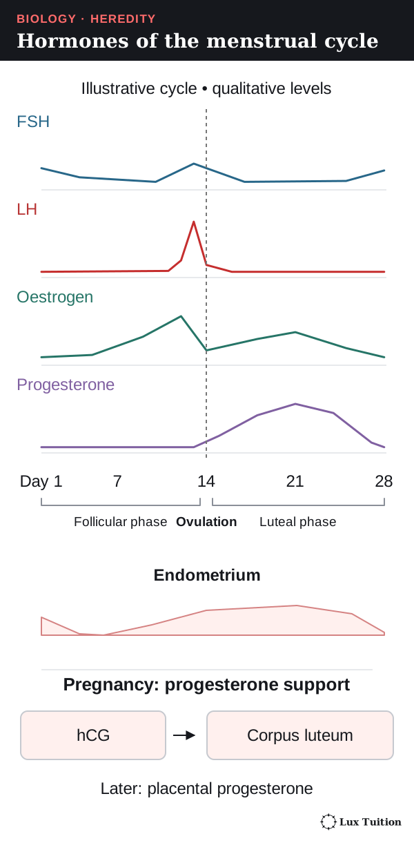
The ovarian and menstrual cycles
The ovarian cycle (changes in the ovary) and menstrual cycle (changes in the endometrium) are coordinated by hormones:
- FSH makes a follicle grow; the follicle secretes oestrogen, which rebuilds the endometrium.
- Sustained high oestrogen switches to positive feedback (a loop that increases a change), causing an LH surge, which triggers ovulation.
- The empty follicle becomes the corpus luteum, which secretes progesterone and oestrogen. During this luteal phase, progesterone maintains a secretory endometrium ready for implantation. These hormones (and inhibin) hold FSH and LH down.
- Without pregnancy, the corpus luteum shrinks, progesterone and oestrogen fall, and the endometrium’s top layer is shed as menstruation. FSH rises and the cycle restarts.
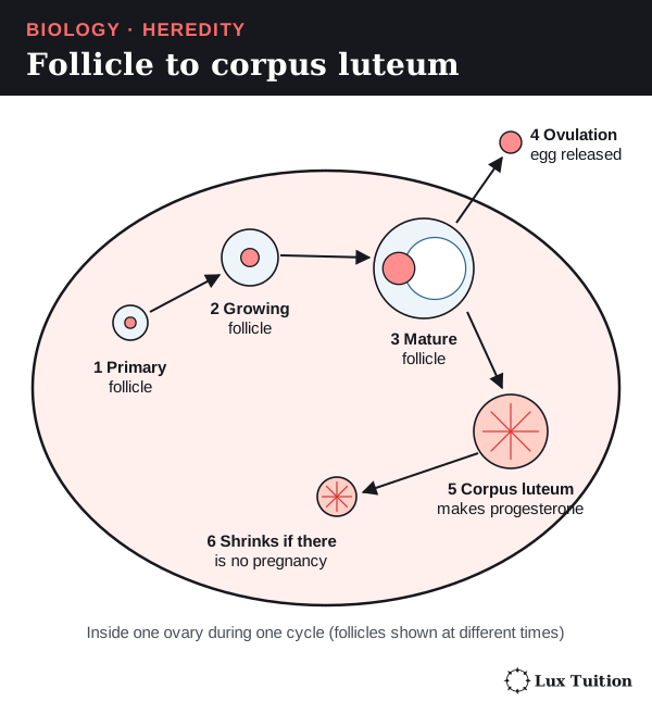
A 28-day diagram is a model, not a fixed timetable. On a hormone graph, the narrow LH peak marks the signal for ovulation and the later progesterone rise shows the corpus luteum at work.
What happens between fertilisation and implantation?
Fertilisation
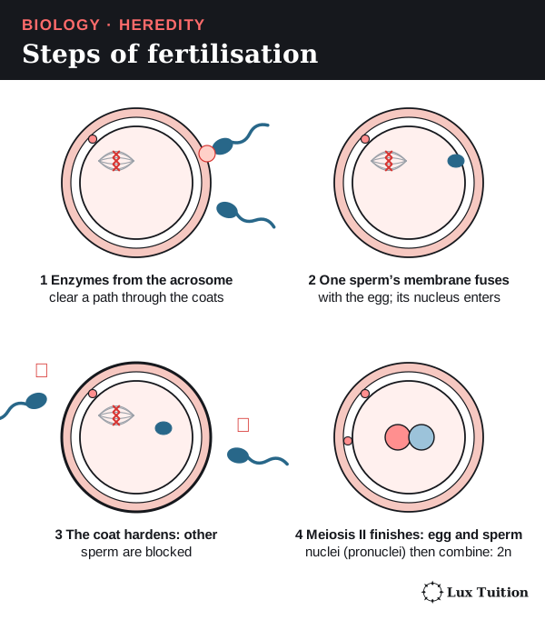
Fertilisation usually happens in the oviduct. The egg is covered by follicle cells and a jelly-like coat, the zona pellucida.
- Sperm change inside the female tract so they can fertilise.
- Enzymes from a sperm’s acrosome clear a path through the follicle cells and zona pellucida.
- One sperm’s membrane fuses with the egg’s, and its nucleus enters.
- The egg’s cortical reaction changes the coat so no more sperm can enter. This block to polyspermy (polyspermy: more than one sperm entering) keeps the chromosome number normal.
- The egg finishes meiosis II, and the two chromosome sets combine in the diploid zygote.
So fertilisation both starts development and combines genetic information from two gametes.
From zygote to implantation
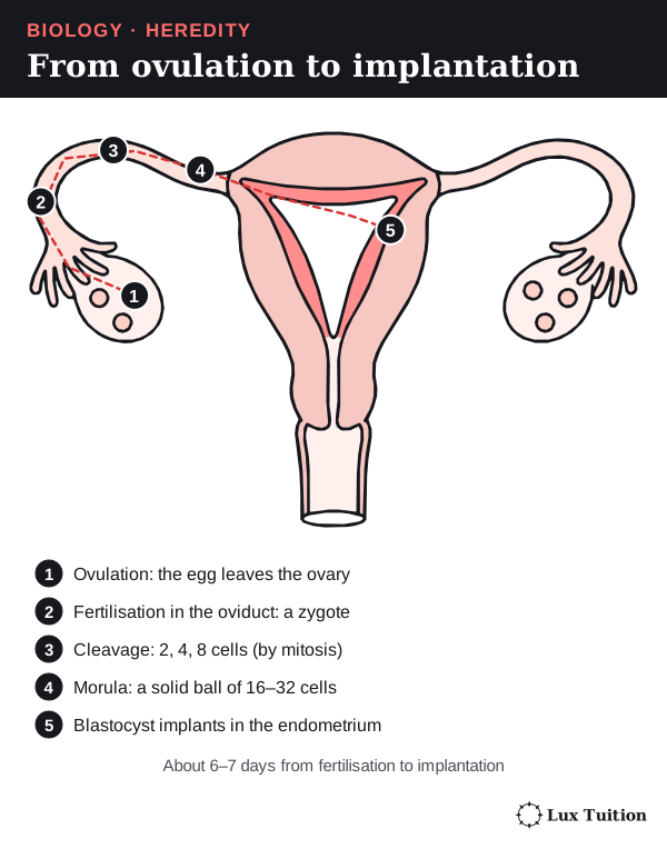
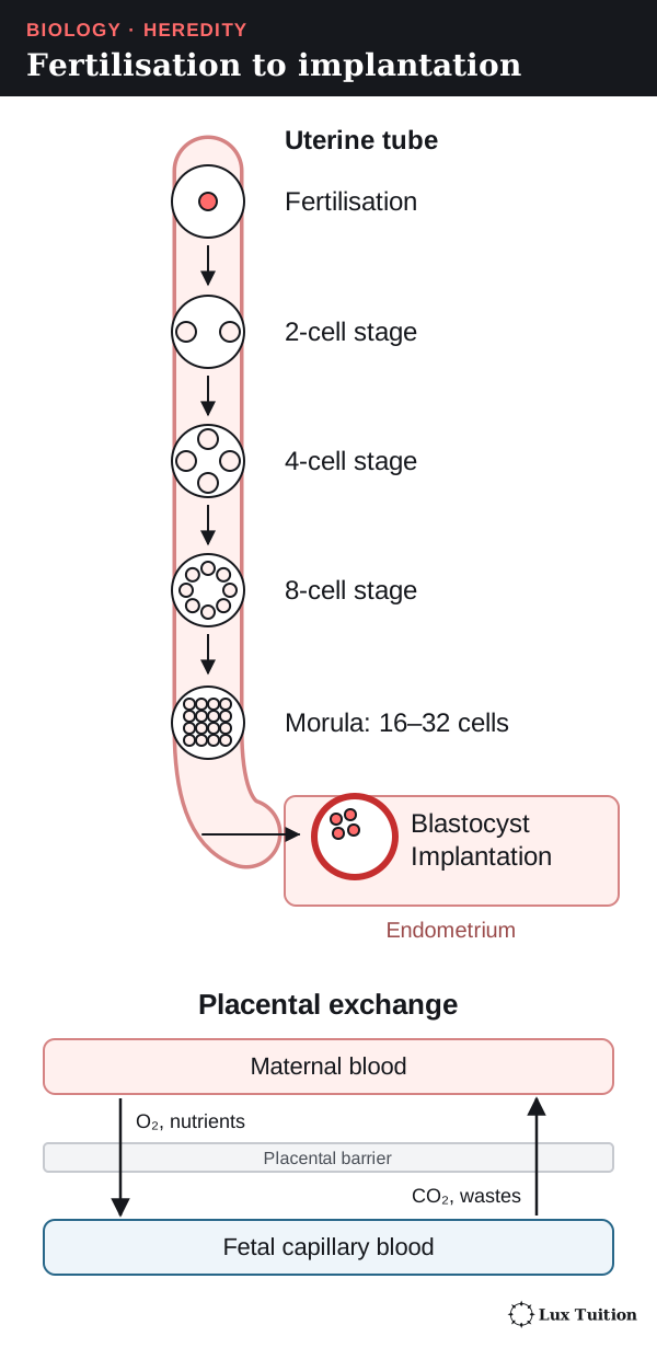
Cleavage is the series of mitotic divisions after fertilisation. The embryo hardly grows at first, so its cells get smaller.
- The zygote divides into 2, 4, 8 cells and so on.
- At about 16–32 cells it is a solid ball, the morula.
- A fluid-filled space forms, making a blastocyst: an inner cell mass (which becomes the embryo) and an outer trophoblast (which forms the embryo’s part of the placenta).
- Implantation: about six to seven days after fertilisation, the blastocyst attaches to the endometrium and its trophoblast cells invade and embed it in the lining, where it can draw nutrients.
The placenta
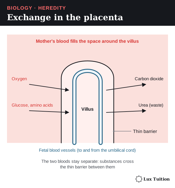
The placenta forms from both embryo and mother. It brings fetal and maternal blood close together, separated by a thin barrier:
- oxygen and nutrients pass to the fetus; carbon dioxide and other wastes pass to the mother
- the two bloods normally do not mix
- finger-like chorionic villi give a huge surface area for exchange
- the placenta also makes hormones that maintain pregnancy.
How do hormones control pregnancy and birth?
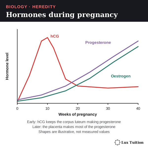
Pregnancy needs the endometrium to stay in place, and progesterone keeps it there. So what keeps progesterone high?
- After implantation, trophoblast cells secrete human chorionic gonadotrophin (hCG).
- hCG keeps the corpus luteum alive, so it keeps making progesterone.
- Later, the placenta makes enough progesterone and oestrogens to take over.
- Progesterone maintains the endometrium and makes the uterus muscle less likely to contract.
- Oestrogens support growth and changes in the mother’s reproductive tissues.
- hCG peaks in the first trimester (three months), then falls, while progesterone and oestrogen keep rising.
hCG is not another name for progesterone: the hormones have different sources and jobs. Endotext’s account of pregnancy endocrinology explains the corpus luteum–placenta handover.
The uterus near birth
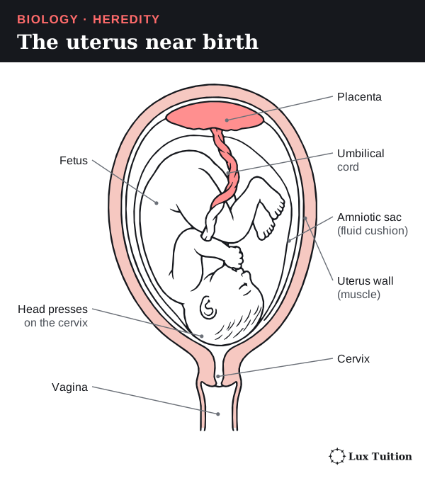
Near birth the fetus usually lies head-down in the fluid-filled amniotic sac, joined to the placenta by the umbilical cord. The muscular uterus wall provides the force for birth, and the cervix must open.
Hormones and birth
Near birth, signals from the fetus, placenta and mother make the uterus more responsive. Prostaglandins (local signalling chemicals) soften the cervix and trigger contractions. In humans the change in progesterone’s effect is called functional withdrawal; blood progesterone does not have to drop suddenly before labour.
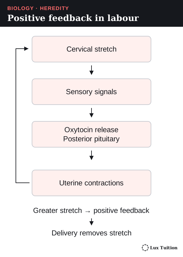
During labour, positive feedback drives contractions:
- The baby stretches the cervix.
- Nerve signals reach the brain, and the posterior pituitary releases oxytocin.
- Oxytocin makes the uterus contract harder, which stretches the cervix more. Back to step 1.
Birth removes the stretch, ending the loop. (Negative feedback, by contrast, reduces a change.)
After birth, oxytocin also triggers milk release, while prolactin drives milk production. Pregnancy is usually dated as about 40 weeks from the last menstrual period, about 38 weeks from fertilisation, so check a timeline’s starting point.
How is plant and animal reproduction manipulated in agriculture?
Selective breeding
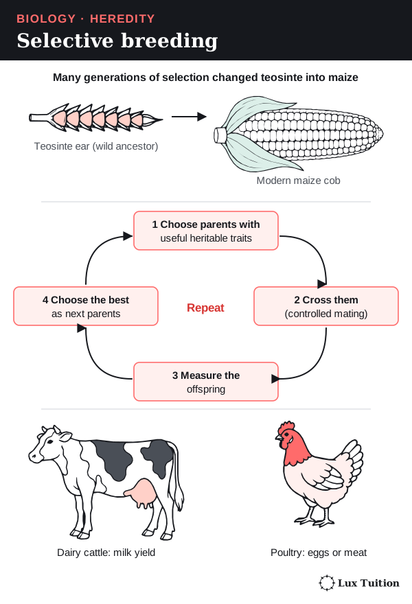
Selective breeding means humans choose which organisms reproduce:
- Choose parents with useful heritable characteristics (ones passed on in the genes).
- Cross them and measure the offspring.
- Choose the best offspring as the next parents, and repeat for many generations.
Selection does not create an allele because it is needed; it changes which existing alleles are passed on. Recombination (shuffling in meiosis and fertilisation) makes new combinations; mutation is the source of new alleles.
Examples: maize was bred from a wild grass, teosinte; poultry are bred for eggs or meat; dairy cattle for milk yield. These are usually complex traits, controlled by many genes and the environment, so a top parent does not guarantee top offspring. Comparing animals on the same feed and management separates inherited from environmental differences.
Methods that manipulate reproduction
| Method | How reproduction is manipulated | Benefit and limitation |
|---|---|---|
| Controlled pollination | Pollen from a chosen parent is placed on a chosen flower, and unwanted pollen is kept out. | Combines the parents’ alleles, but the offspring vary and may not get the wanted combination. |
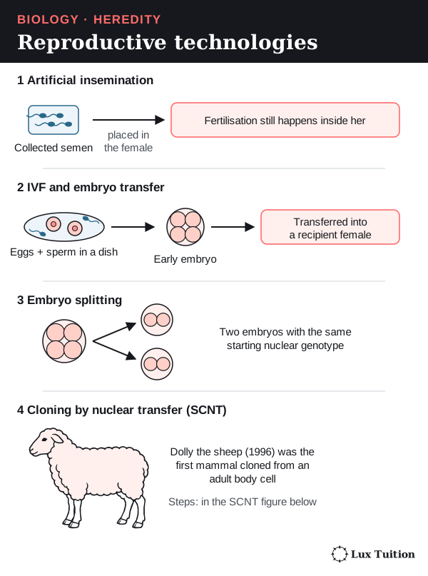
| Artificial insemination | Collected semen is placed in a female’s reproductive tract at the right time. Fertilisation still happens inside her. | One chosen male can father many offspring, and semen can be stored; overusing a few males reduces genetic diversity. |
| IVF and embryo transfer | Eggs are fertilised outside the body (in vitro means “in glass”); early embryos are transferred into other females. | More offspring can come from chosen parents, but it needs expertise, resources and proper animal care. |
| Embryo splitting | The cells of an early embryo are separated to make embryos with the same starting nuclear genotype. | Copies a valuable combination, but makes no new combinations and does not remove environmental differences. |
| Cuttings and tissue culture | Plant cells divide by mitosis; in suitable conditions they grow roots, shoots or whole plants. | Quickly produces many copies of a useful plant; one disease or shared weakness can affect all these similar plants. |
| Grafting | A shoot (the scion) from one plant is joined onto the roots (the rootstock) of another plant. | Combines a useful rootstock and a useful shoot without mixing their DNA into a new hybrid. |
Cloning by somatic cell nuclear transfer
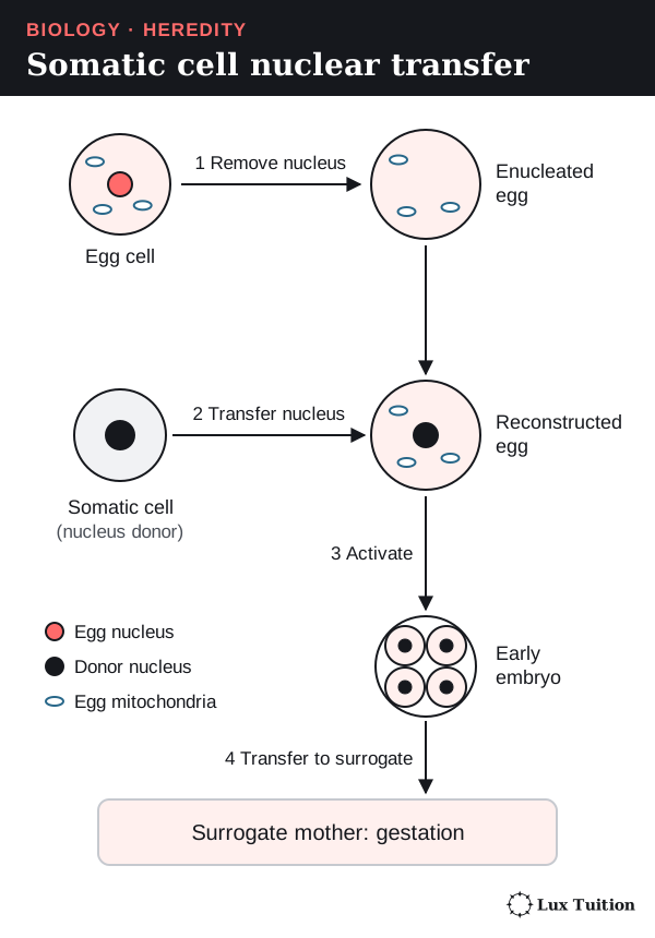
A somatic cell is any body cell that is not a gamete. In somatic cell nuclear transfer (SCNT):
- Remove the nucleus from an egg cell.
- Insert the nucleus of a somatic cell.
- Stimulate the egg to divide into an embryo.
- Transfer the embryo to a surrogate mother.
Dolly the sheep was cloned from the nucleus of an adult mammary cell. Her nuclear DNA came mainly from the nucleus donor, and her mitochondrial DNA (DNA in the mitochondria) mainly from the egg donor. Development, gene regulation, epigenetic state (chemical marks that switch genes on or off) and environment mean a clone need not be identical in every characteristic. Roslin Institute’s account of Dolly.
Polyploidy: making new crops
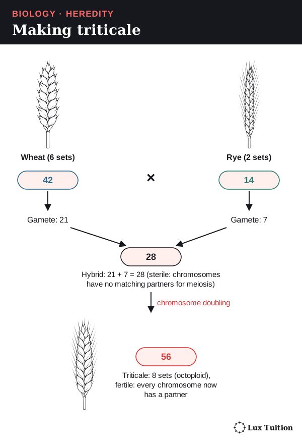
Polyploidy means more than two complete chromosome sets. A hybrid of two species is often sterile (cannot reproduce) because its chromosomes have no matching partners in meiosis. Doubling every chromosome gives each a partner and can restore fertility. Triticale (a wheat–rye crop):
- Hexaploid wheat (6 sets, 42 chromosomes) makes gametes with 21.
- Diploid rye (2 sets, 14) makes gametes with 7.
- The hybrid has 21 + 7 = 28 chromosomes and is sterile.
- Doubling gives octoploid (8 sets) triticale with 56.
Hexaploid triticale varieties (42 chromosomes) also exist. The number in one basic set is written x, to avoid confusion with n, the number in a gamete. Odd numbers of sets often upset meiosis, but polyploidy does not always cause sterility.
Weighing up the methods
- Fast multiplication and uniform crops or herds can raise production.
- Inbreeding (breeding close relatives) increases homozygosity and can expose harmful recessive alleles (alleles that only show their effect when no dominant allele is present).
- Low genetic diversity leaves a population vulnerable to a changing environment or a shared disease weakness; diverse breeding stock and seed banks protect future options.
A technique that produces many offspring is not automatically sustainable.
The same chain explains unusual traits in isolated populations (such as on an island): isolation means little gene flow (movement of alleles between populations), so relatives are more likely to mate (inbreeding) → offspring are more likely to inherit two copies of the same recessive allele → rare recessive traits appear more often.
How important is it for genetic material to be replicated exactly?
How are chromosomes and genes copied during the cell cycle?
Before a cell divides, it must copy its DNA exactly so each new cell gets a full set of instructions. More precise vocabulary:
- A gene’s product is a polypeptide (a chain of amino acids that forms all or part of a protein) or a functional RNA molecule (an RNA that does a job itself, such as tRNA, a small RNA that carries amino acids).
- A locus (plural: loci) is the position of a gene on a chromosome.
- Homologous chromosomes are a matching pair, one from each parent, carrying the same genes at the same loci but possibly different alleles.
- Sister chromatids are the two DNA molecules of a copied chromosome, identical except for copying errors, joined at the centromere until they separate.
Homologues come from two parents; sister chromatids are copies of one chromosome. In eukaryotes, each DNA molecule is wound around ball-shaped proteins called histones, then coiled further, which packs it into the nucleus.
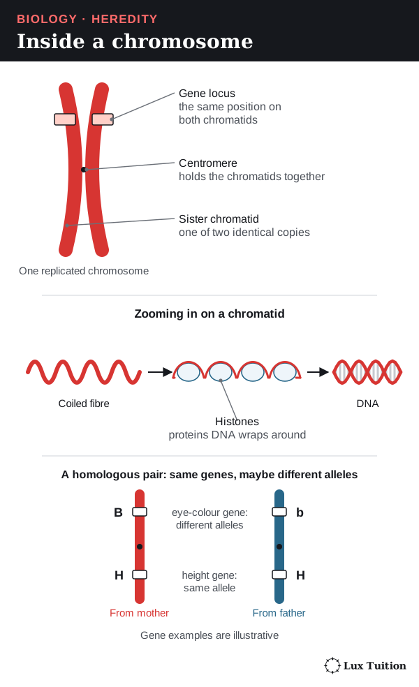
Before copying, a chromosome is one DNA molecule (an I shape); after copying it has two sister chromatids (an X shape). Chromosomes are counted by centromeres, so copying doubles the DNA but not the chromosome number.
The cell cycle
The cell cycle is the sequence of stages from one division to the next:
- G1: the cell grows and does its normal jobs.
- S phase: the DNA is replicated (copied).
- G2: the cell grows and prepares to divide.
- Mitosis separates the copied chromosomes into two nuclei; cytokinesis divides the cytoplasm.
G1, S and G2 make up interphase. Some specialised cells stop dividing altogether.
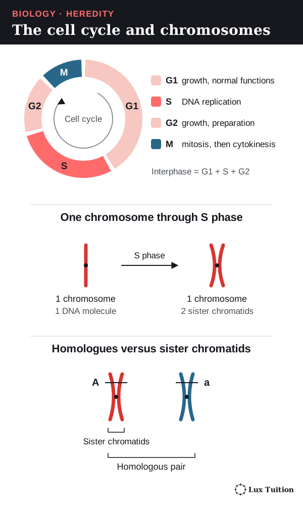
In the table, C is the amount of DNA compared with one unreplicated haploid set, and n is the number of chromosome sets. It compares finished cells, skipping the moment in anaphase when an undivided cell briefly has double the chromosome count.
| Stage in a typical human diploid cell | Chromosomes per cell | Chromatids/DNA molecules per cell | DNA amount |
|---|---|---|---|
| G1 | 46 | 46 | 2C |
| After S phase, before chromosome separation | 46 | 92 | 4C |
| Each daughter cell after mitosis and cytokinesis | 46 | 46 | 2C |
| Each cell after meiosis I and cytokinesis | 23 | 46 | 2C |
| Each product after meiosis II and cytokinesis | 23 | 23 | 1C |
How does mitosis preserve genetic information?
mitosis and meiosis (ACSBL075)
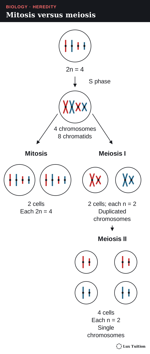
Mitosis happens after the DNA is copied in S phase. The spindle is a set of protein fibres (microtubules) stretching between the two poles (ends) of the cell; spindle fibres attach to a protein patch on each centromere, the kinetochore.
- Prophase: chromosomes condense, the spindle forms, the nuclear envelope breaks down and fibres attach to kinetochores.
- Metaphase: copied chromosomes line up one by one across the equator.
- Anaphase: sister chromatids separate to opposite poles; each is now a chromosome.
- Telophase: nuclear envelopes re-form and the chromosomes uncoil.
Cytokinesis then divides the cytoplasm: animal cells pinch in (a cleavage furrow); plant cells build a cell plate.
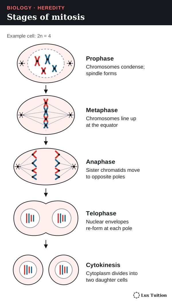
Each new nucleus normally gets one copy of every chromosome, so mitosis keeps the chromosome number and genetic information the same. It allows growth, repair, cell replacement and many kinds of asexual reproduction, in haploid as well as diploid cells. The products are not guaranteed identical: mutations and errors in separating chromosomes can occur.
How does meiosis produce haploid cells?
Meiosis has one round of DNA copying followed by two divisions. In animals it makes cells that become gametes; in plants it makes spores, and gametes form later by mitosis.
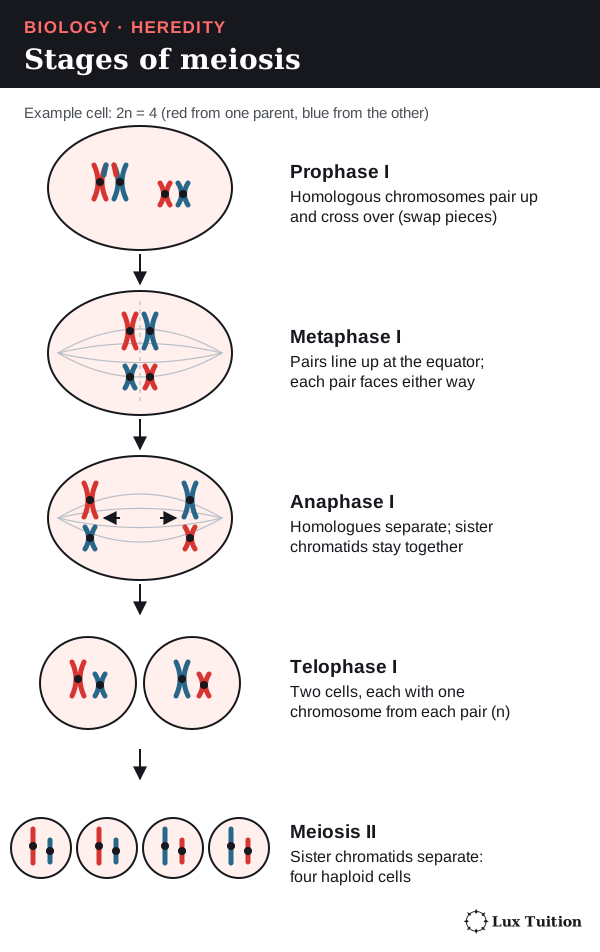
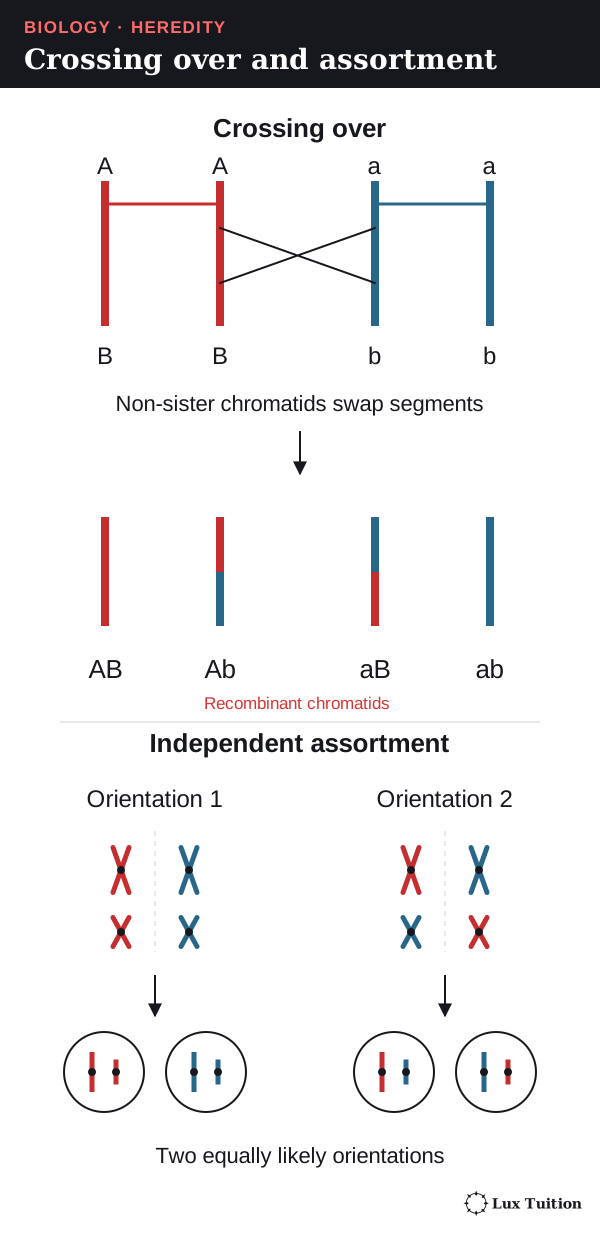
- Prophase I: homologous chromosomes pair up. In crossing over, matching DNA segments are swapped between non-sister chromatids (one from each homologue), making recombinant chromatids with new allele combinations.
- Metaphase I: pairs line up at the equator; each pair’s orientation is independent of the others.
- Anaphase I: homologues separate; sister chromatids stay together.
- Telophase I and cytokinesis: two haploid cells form, each chromosome still with two chromatids. The DNA is not copied again.
- Meiosis II: sister chromatids separate, much like mitosis, giving four cells, each with one chromosome from each original pair.
| Feature | Mitosis | Meiosis |
|---|---|---|
| Nuclear divisions | One | Two |
| Homologue pairing and normal crossing over | Absent | Present in prophase I |
| First separation | Sister chromatids | Homologous chromosomes |
| Chromosome-set number | Kept the same | Halved |
| Typical products | Two nuclei with the parent’s chromosomes | Four haploid nuclei; whether they become gametes depends on the organism |
| Main job | Genetic continuity in growth, repair and asexual reproduction | Balanced sexual life cycles and new combinations of alleles |
When meiosis goes wrong: nondisjunction
Nondisjunction is when chromosomes fail to separate properly in meiosis.
- In meiosis I, a homologous pair fails to separate; in meiosis II, two sister chromatids fail to separate.
- Either way, one gamete gets an extra copy of that chromosome and another gamete gets no copy.
Fertilisation then completes the error. For example, if nondisjunction of the sex chromosomes leaves a sperm or egg with no sex chromosome, and it fuses with a normal gamete carrying an X, the zygote has only one sex chromosome: 45,X (Turner syndrome).
So an explanation needs both steps: the wrong number of chromosomes is made in meiosis, then passed into the zygote at fertilisation.
How does DNA structure allow complementary base pairing?
DNA replication using the Watson and Crick DNA model, including nucleotide composition, pairing and bonding (ACSBL076, ACSBL077)
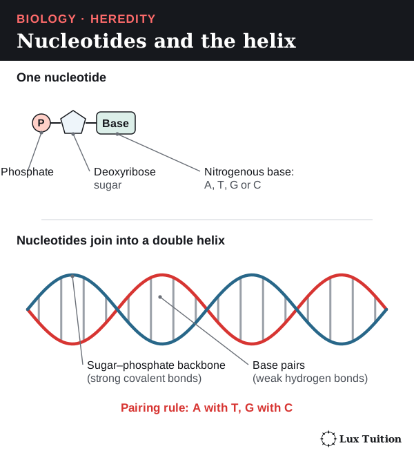
DNA is built from units called nucleotides, each with a phosphate group, a deoxyribose sugar and one nitrogenous base: adenine (A), thymine (T), guanine (G) or cytosine (C).
- Covalent bonds (strong bonds made by sharing electrons) called phosphodiester bonds join the sugar of one nucleotide to the phosphate of the next, forming each strand’s sugar–phosphate backbone.
- The bases point inwards. Hydrogen bonds (weak attractions) hold the bases of the two strands together.
- Complementary base pairing: A pairs with T (two hydrogen bonds); G pairs with C (three).
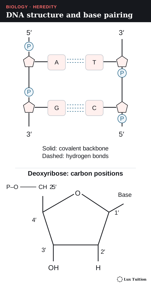
The strands are antiparallel: one runs 5′ to 3′, its partner 3′ to 5′. The numbers name carbon atoms in the sugar, so they show which way a strand points.
- Complementary pairing keeps the helix the same width.
- Each strand can be a template (pattern) for rebuilding the other.
- Information is stored in the sequence (order) of bases.
| Strand | Sequence |
|---|---|
| One DNA strand | 5′–ATGC–3′ |
| Complementary strand | 3′–TACG–5′ |
The Watson–Crick double-helix model explains how complementary templates allow copying. A flat ladder diagram shows pairing and direction but not the 3D twist, real size or protein interactions.
How does semiconservative DNA replication work?
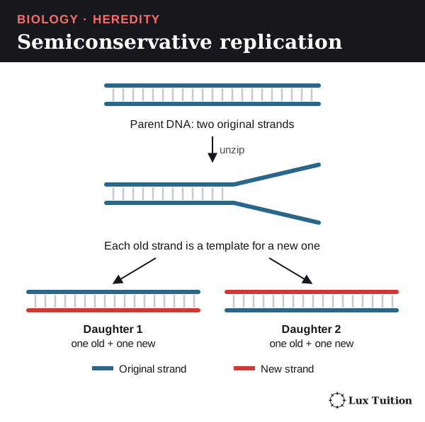
DNA replication is semiconservative: each new molecule keeps one original strand and gains one new strand. It happens in S phase, before mitosis and before meiosis I.
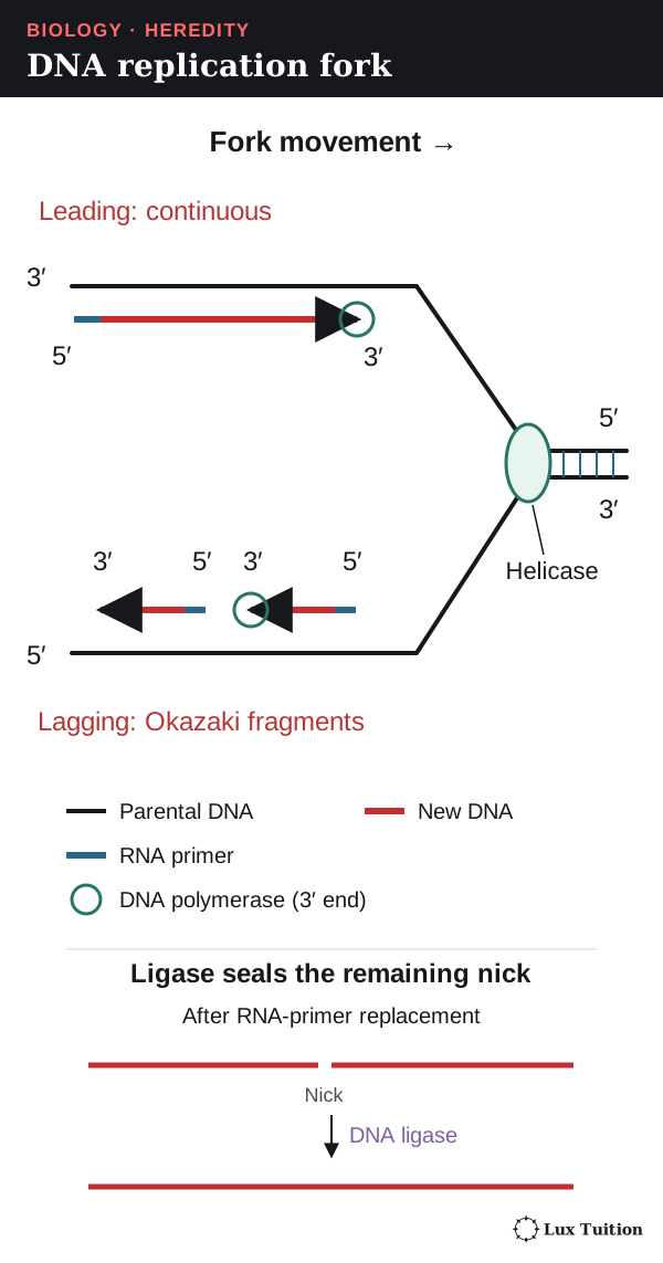
Enzymes work together at the replication fork, where the helix is opening:
- Helicase unzips the helix by breaking hydrogen bonds between base pairs.
- Topoisomerases relieve twisting strain ahead of the fork; single-strand binding proteins keep the strands apart.
- Primase makes short RNA primers (short starter pieces of RNA that pair with the template), giving DNA polymerase a free 3′ end: an exposed 3′ hydroxyl (–OH) group on the sugar, the chemical hook the next nucleotide bonds to.
- DNA polymerase adds complementary nucleotides, building 5′ to 3′ while reading the template 3′ to 5′. Its building blocks are nucleotide triphosphates (nucleotides carrying three phosphate groups); each joining step uses two of those phosphates as an energy source and releases them as pyrophosphate.
Because the templates run in opposite directions:
- the leading strand is made continuously, towards the moving fork
- the lagging strand is made in short Okazaki fragments, each built 5′ to 3′ away from the fork
- RNA primers are replaced by DNA, and DNA ligase seals the gaps. Ligase joins fragments; it does not choose bases or unzip the helix.
Pairing, proofreading and repair make copying very accurate but not perfect. An unrepaired change becomes a mutation, which may be neutral, harmful or helpful. A mutation in a germline cell (one that makes gametes) can reach offspring; in sexual reproduction, an ordinary mutation in a somatic (body) cell generally stays within that individual’s cell lineage.
Types of mutation
A point mutation changes a single base. The commonest is a substitution (one base swapped for another). Its effect depends on the codon it changes (a codon is three bases of mRNA (messenger RNA, the gene’s working copy) that specify an amino acid or a stop signal; see the translation section):
- Silent: the new codon codes for the same amino acid (GUC → GUU, both valine), so the protein is unchanged.
- Missense: the new codon codes for a different amino acid. GUC → AUC changes valine (Val) to isoleucine (Ile).
- Nonsense: the new codon is a stop codon (UAC → UAA), so the protein is cut short.
An insertion or deletion adds or removes bases. Because codons are read in threes, adding or removing one or two bases shifts every codon after it (a frameshift), usually changing many amino acids.
A new mutation in a germline cell can be traced forward. Worked model for an autosomal gene (one on a non-sex chromosome):
- A germline cell is AA. Before DNA replication, one A changes to a new allele, a*. The cell is now Aa*.
- Meiosis separates the two alleles, so half the gametes from that cell line carry A and half carry a*. (Other germline cells without the mutation still make only A gametes, so overall fewer than half of the parent’s gametes carry a*.)
- Fertilisation by an A gamete from the other parent gives AA offspring (if the egg or sperm carried A) or Aa* offspring (if it carried a*).
An Aa* offspring is heterozygous (has two different alleles at that locus). It carries the new allele in every cell, because all its cells come from that zygote. (For an X-linked gene, an XY offspring has only one copy, so it would carry a* alone.)
How cell replication supports the continuity of species
DNA replication copies the DNA, mitosis shares the copies between cells, meiosis halves the chromosome number before gametes fuse, and fertilisation restores it. Variation lets different allele combinations survive in different conditions; it does not guarantee survival. Variation does not make every offspring unique at every locus.
Why is polypeptide synthesis important?
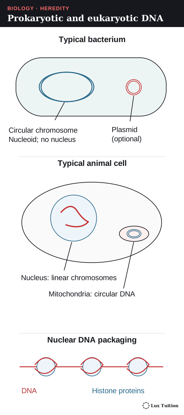
How does DNA differ in prokaryotes and eukaryotes?
Start here: from DNA to protein
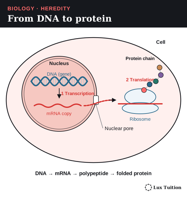
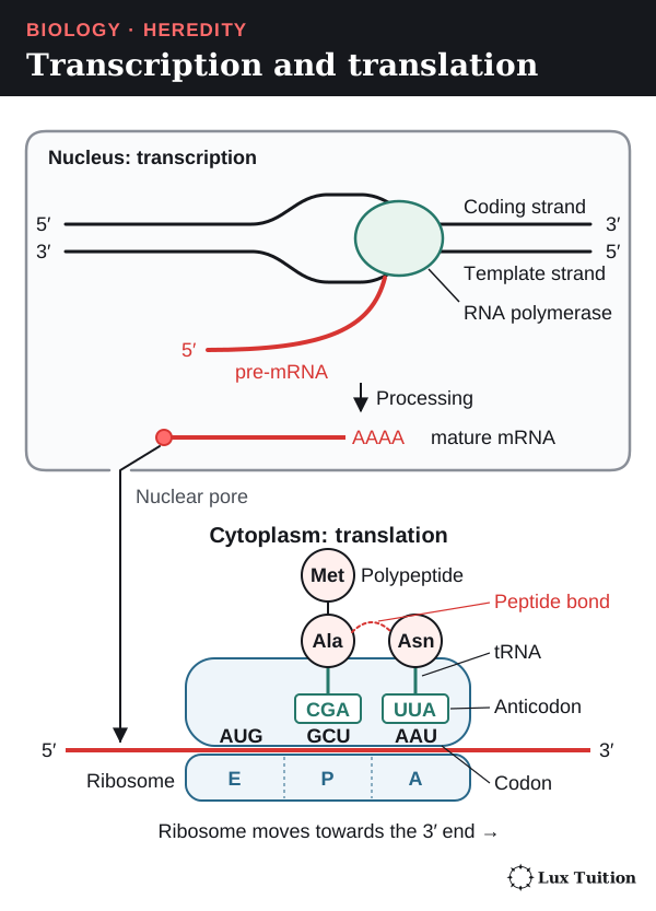
Polypeptide synthesis (protein synthesis) uses a gene’s instructions in two steps:
- Transcription: the gene is copied into mRNA (messenger RNA). In eukaryotes this happens in the nucleus.
- Translation: a ribosome (a small protein-building structure) reads the mRNA and joins amino acids in order.
RNA uses the sugar ribose and the base uracil (U) instead of thymine (T).
How DNA is stored in prokaryotes and eukaryotes
| Feature | Typical bacterial cell | Typical eukaryotic cell |
|---|---|---|
| Main location | Nucleoid region, with no nuclear envelope | Chromosomes enclosed in a nucleus |
| Main chromosome form | Usually one circular double-stranded DNA molecule | Several linear (straight) double-stranded DNA molecules |
| Packaging | Held by DNA-binding proteins | Wrapped around histone proteins to form chromatin (the DNA–protein mix that makes up chromosomes) |
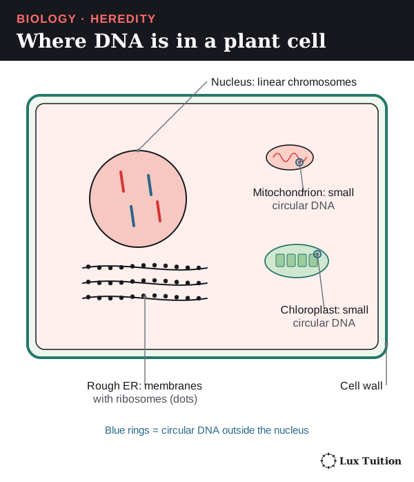
| Extra DNA | Plasmids may be present | Mitochondria, and chloroplasts in plants and algae, have their own DNA |
| Gene expression | Transcription and translation can happen together | Transcription (in the nucleus) is separate from translation (in the cytoplasm) |
These are typical models: archaea are also prokaryotes and many have histone proteins; some bacteria have more than one chromosome or linear ones, not all carry plasmids, and not every plasmid carries useful genes such as antibiotic resistance.
What is in a eukaryotic gene?
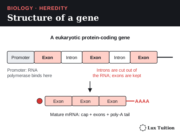
A protein-coding gene has:
- a promoter, a control sequence just before the gene where RNA polymerase (the enzyme that builds RNA) and its helper proteins bind to start transcription (not the same as the start codon, the signal where translation begins)
- exons, the sections kept in the finished mRNA (exons can include untranslated regions at the ends that are kept in the mRNA but never read into amino acids)
- introns, the sections removed before the mRNA leaves the nucleus.
How does transcription produce and process RNA?
transcription and translation
In transcription:
- RNA polymerase recognises the promoter.
- It separates the DNA strands in a small region.
- It adds complementary RNA nucleotides, reading the template strand 3′ to 5′ while the RNA grows 5′ to 3′ (template A pairs with U, T with A, C with G).
- It stops at termination signals in the DNA, not at a stop codon (a translation signal, covered below).
Only one strand is the template for a given gene. The other, the coding strand, matches the RNA when both are written 5′ to 3′, except that DNA has T where RNA has U. Different genes can use different strands.
Processing the RNA (eukaryotes)
The first copy, pre-mRNA, is processed in the nucleus:
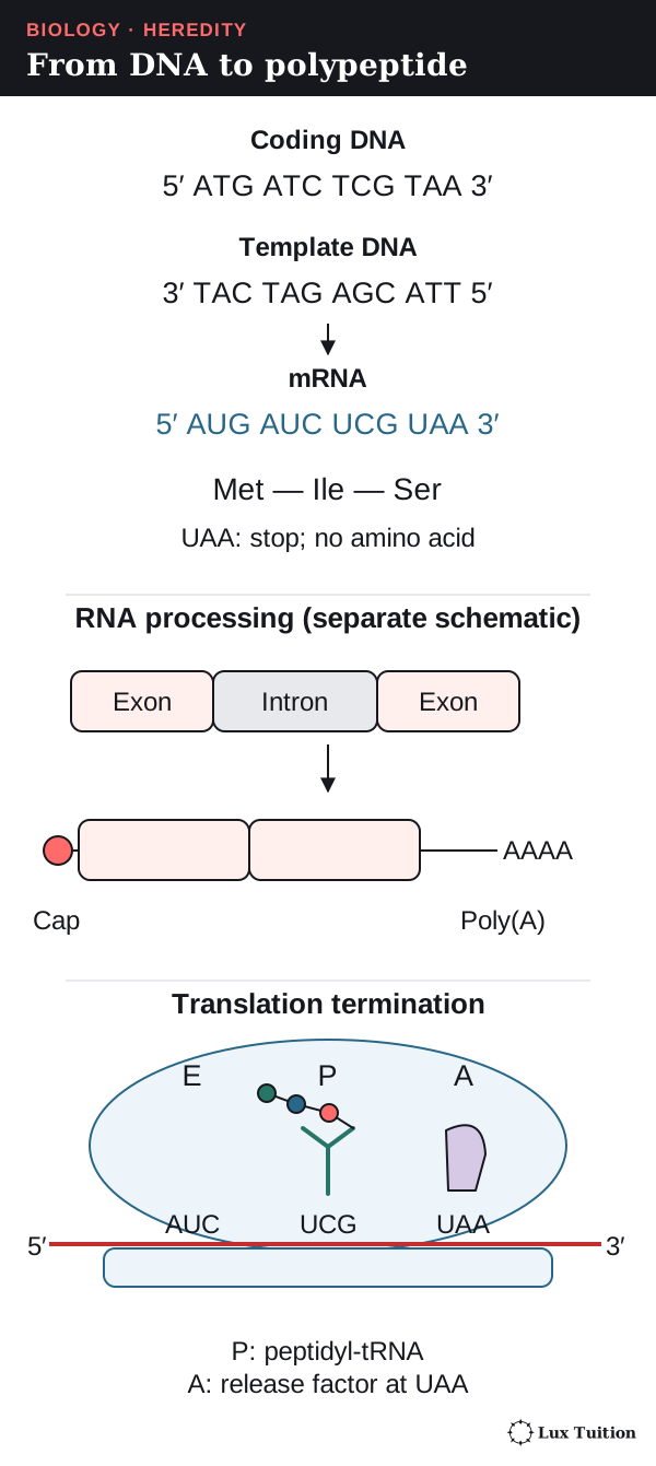
- a 5′ cap and usually a 3′ poly-A tail (a string of A nucleotides) are added; they protect the RNA and help export and translation
- splicing removes introns and joins exons
- alternative splicing joins exons in different combinations, so one gene can give several mature mRNAs and polypeptides.
Mature mRNA leaves through nuclear pores and is translated by free ribosomes or by ribosomes on the rough endoplasmic reticulum (a membrane network studded with ribosomes).
How does translation turn mRNA codons into a polypeptide?
assessing the importance of mRNA and tRNA in transcription and translation (ACSBL079)
The genetic code
mRNA is read in groups of three bases called codons, read 5′ to 3′.
- Of the 64 codons, 61 code for amino acids and three (UAA, UAG, UGA) are stop codons that end the chain.
- AUG codes for methionine and is normally the start codon, where translation begins.
- The code is degenerate (several codons can code for one amino acid), unambiguous (each codon has one meaning) and nearly universal (with exceptions such as some mitochondrial codes).
tRNA (transfer RNA) is a small folded RNA that carries an amino acid at one end and an anticodon (three bases that pair with a codon) at the other.
| Component | Job |
|---|---|
| mRNA | Carries the ordered codons that act as the template for translation. |
| tRNA | Acts as an adaptor between codon and amino acid. |
| Aminoacyl-tRNA synthetases | Enzymes that attach the correct amino acid to each tRNA: a crucial accuracy step. |
| Ribosome and rRNA | Holds the mRNA and tRNAs in place; ribosomal RNA (rRNA) catalyses (speeds up) the bonding of amino acids (peptide bonds). |
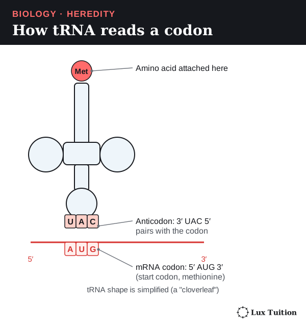
The anticodon pairs antiparallel to the codon: mRNA 5′–AAU–3′ pairs with 3′–UUA–5′ and codes for asparagine. Flexible pairing at the third position (wobble) lets some tRNAs read more than one codon, so there need not be 61 kinds of tRNA.
Translation step by step
The ribosome holds tRNAs in three sites: A (arriving), P (holding the growing chain) and E (exit).
- Initiation: the ribosome and the first tRNA (methionine) assemble at the start codon.
- Elongation: a tRNA with the next amino acid enters the A site, pairing with the next codon.
- A peptide bond (the link between amino acids) joins it to the chain held in the P site.
- The ribosome moves one codon: the chain-bearing tRNA shifts from A to P, and the empty tRNA leaves from the E site. Steps 2–4 repeat.
- Termination: at a stop codon, a release factor (a protein, not a tRNA) frees the chain.
The chain grows from its amino end (–NH₂) to its carboxyl end (–COOH). The simplified example below is an uninterrupted coding region, not a complete eukaryotic gene, and shows how strands and product relate.
| Molecule | Sequence or product |
|---|---|
| Coding DNA | 5′–ATG ATC TCG TAA–3′ |
| Template DNA | 3′–TAC TAG AGC ATT–5′ |
| mRNA | 5′–AUG AUC UCG UAA–3′ |
| Translation | Methionine–isoleucine–serine, then termination |
Why cells need polypeptide synthesis
analysing the function and importance of polypeptide synthesis (ACSBL080)
“Stop” is not an amino acid. A chain can start folding while it is being made, and some proteins need chemical modification, processing or other chains before they work. Polypeptide synthesis links the inherited DNA sequence to the enzymes, receptors (signal-receiving proteins) and structural proteins a cell needs; a gene is useless if its product cannot be made correctly.
How do genes and environment affect phenotype?
assessing how genes and environment affect phenotypic expression (ACSBL081)
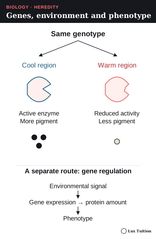
An organism’s genotype is its alleles at the genes being studied; its phenotype is its observable or measurable characteristics. A phenotype depends on many genes, on how strongly they are switched on (gene expression), on the environment, and on their interactions. Specialised cells share essentially the same genome (full set of DNA) but switch on different genes.
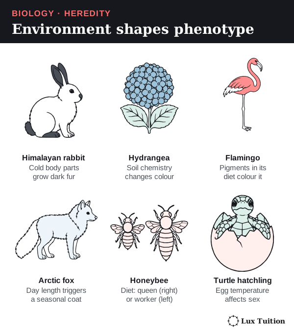
| Example | How genes and environment combine to give the phenotype |
|---|---|
| Human height | Many genetic variants affect growth, while nutrition, health and other conditions affect the final height. It is not a single dominant/recessive trait. |
| Skin pigmentation | Several genes affect pigment production; ultraviolet (UV) light can increase pigment production in an individual. Tanning does not need any inherited change in DNA sequence. |
| Hydrangea flower colour | In responsive varieties, soil conditions change how much aluminium the plant can take up, which changes the pigment’s colour. Soil pH works through this chemistry; it does not rewrite flower-colour genes. |
| Himalayan rabbit pigmentation | A temperature-sensitive enzyme that makes pigment works better in cooler body parts, so the ears, nose, feet and tail are darker. This shows changed protein activity, not necessarily an epigenetic switch (a change in gene regulation without a change in DNA sequence). |
| Flamingo colour | Carotenoid pigments from the diet colour the feathers; genes affect how those pigments are processed. |
| Seasonal arctic fox coat | Seasonal signals, especially photoperiod (day length), control moulting and coat features through the body’s own regulation. |
Honeybees. Whether a female larva becomes a queen or a worker depends on diet and gene regulation. A 2008 experiment by Kucharski and colleagues reduced a DNA-methylation enzyme (methylation is a chemical tag that helps switch genes off) in larvae, and more developed queen features. This supports a role for gene regulation; it does not mean every diet effect works through methylation, or that all bees in a hive are genetically identical.
Turtles. In red-eared slider turtles, egg incubation temperature affects whether a hatchling develops as male or female. Ge and colleagues’ 2018 study linked this to regulation of the genes KDM6B and Dmrt1. It is not a rule for all reptiles.
The environment can change gene expression or protein activity without changing DNA sequence; a mutation changes the sequence itself. These are different mechanisms, and mutations can alter proteins or regulation with effects that depend on environmental conditions.
How does protein structure determine function?
Every amino acid has a central carbon carrying an amino group (–NH₂), a carboxyl group (–COOH), a hydrogen atom and an R group (side chain) that differs between the 20 amino acids. A peptide bond joins the carboxyl group of one to the amino group of the next.
The R groups decide how the chain folds and what it binds.
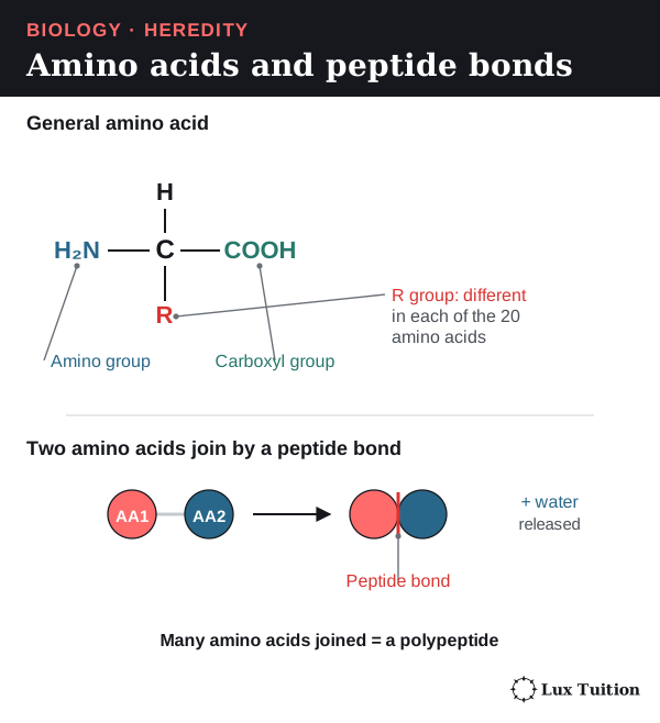
Four levels of structure
Three bonds in the table need defining: hydrophobic interactions (water-avoiding R groups clustering together inside the protein), ionic bonds (attractions between oppositely charged R groups) and disulfide bonds (strong covalent links between sulfur-containing R groups).
| Structural level | What it means and what holds it together | Why it matters |
|---|---|---|
| Primary | The sequence (order) of amino acids, linked by covalent peptide bonds | Decides which side chains are at each position. |
| Secondary | Local coils (alpha helices) and folds (beta sheets), held by hydrogen bonds between backbone groups | Gives repeating shapes within the chain; these bonds are mainly not between R groups. |
| Tertiary | The overall 3D shape of one polypeptide, held by hydrophobic interactions, hydrogen bonds, ionic bonds and sometimes disulfide bonds | Positions an enzyme’s active site or a receptor’s binding region. |
| Quaternary | Two or more polypeptide chains fitted together | Lets chains work as a team, as in haemoglobin; not all proteins have this level. |

Shape decides function
An enzyme’s active site is a pocket whose shape and chemical properties let only its substrate (the molecule it acts on) bind. Binding lowers the activation energy (the energy needed to start the reaction), so the reaction speeds up.
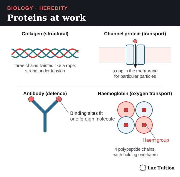
- Collagen forms rope-like fibres that give tissues strength.
- Channel proteins form gaps in membranes for particular particles.
- Antibodies, made by the immune system, have binding sites that fit particular foreign molecules.
- Haemoglobin carries oxygen in red blood cells. It has four polypeptide chains and four haem groups; the haem groups are not extra chains.
Denaturation
Heat or a change in pH can break the weak interactions holding a protein’s shape. This denaturation loses the shape and function, though the peptide bonds and primary sequence usually stay intact. The conditions that denature a protein vary between proteins, and denaturation is not always permanent.
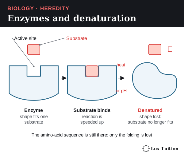
How can the genetic similarities and differences within and between species be compared?
How meiosis and fertilisation create genetic variation
Three processes make offspring genetically different:
- Independent assortment: in metaphase I each homologous pair lines up independently, so gametes get a random mix of maternal and paternal chromosomes. With n pairs there are up to 2n combinations (before crossing over). Two genes on different homologous pairs give AB, Ab, aB and ab; humans have 223, about 8.4 million, possible combinations across many meioses.
- Crossing over can separate alleles on the same chromosome: from AB and ab homologues it can make Ab and aB chromatids. It makes new combinations, not new alleles.
- Random fertilisation joins any gamete from one parent with any from the other, restoring the diploid number and multiplying the possible genotypes.
How do segregation and dominance affect inheritance?
interpreting examples of autosomal, sex-linkage, co-dominance, incomplete dominance and multiple alleles (ACSBL085)
Mendel’s experiments
Gregor Mendel found the basic rules of inheritance with garden peas. He chose easily distinguished traits (seed colour, seed shape), started from true-breeding lines (plants that always produce offspring like themselves), controlled pollination, and counted large numbers of offspring.
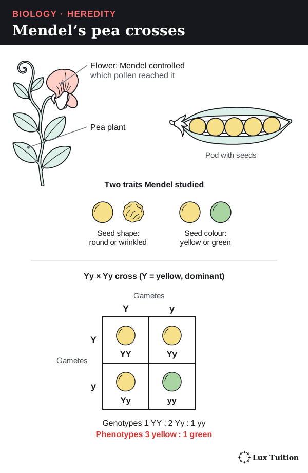
Mendel’s law of segregation: each parent has two copies of a gene, and they separate into different gametes, because homologues separate in meiosis. Independent assortment applies only to genes that assort independently; linkage (covered below) is the exception.
- Homozygous: two identical alleles (YY or yy). Heterozygous: two different alleles (Yy).
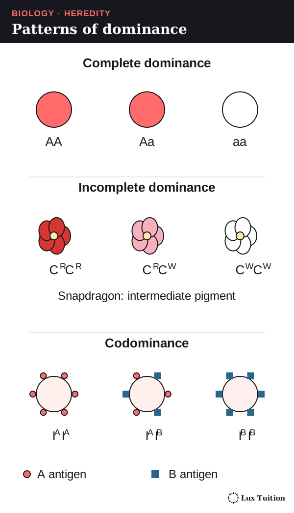
- A dominant allele shows its effect with one copy (capital letter, Y); a recessive allele (lower case, y) only shows when no dominant allele is present: two copies for an autosomal gene, or one copy on the single X of an XY male.
- Under complete dominance, a heterozygote looks like the dominant homozygote. “Dominant” does not mean more common or better.
Punnett squares
A Punnett square shows all the ways two parents’ gametes can combine. With Y (yellow) dominant to y (green), a Yy parent makes Y and y gametes equally often:
| Y gamete | y gamete | |
|---|---|---|
| Y gamete | YY | Yy |
| y gamete | Yy | yy |
The expected ratios are 1 YY : 2 Yy : 1 yy and 3 yellow : 1 green (assuming complete dominance and equal survival). Each offspring is a separate chance event, so four offspring need not match the square exactly.
A test cross with a homozygous recessive (yy) tests a dominant-looking parent: any yy offspring prove it is Yy, but a few all-dominant offspring do not prove YY.
Two genes at once
Multiply probabilities for independent events. In YyRr × YyRr (R = round, r = wrinkled), each parent makes YR, Yr, yR and yr gametes, each 1/4, so P(yyrr) = 1/4 × 1/4 = 1/16.
The 9 : 3 : 3 : 1 ratio assumes independent assortment, complete dominance at both genes and no survival or gene-interaction effects. Human height and hair colour are not simple two-gene examples.
How do incomplete dominance, codominance and multiple alleles compare?
Incomplete dominance
In incomplete dominance the heterozygote is in between. Red snapdragons (CRCR) crossed with white (CWCW) give pink (CRCW); pink × pink gives 1 red : 2 pink : 1 white (1 CRCR : 2 CRCW : 1 CWCW). The alleles stay separate; they do not blend.
Codominance and multiple alleles
In codominance both alleles’ products show fully in the heterozygote. In the ABO blood group, the products are antigens (molecules on red blood cells that the immune system can recognise). The population has three alleles (multiple alleles): IA (A antigen), IB (B antigen) and i (neither). IA and IB are codominant and both dominant to i; each person carries only two.
| Genotype | ABO phenotype |
|---|---|
| IAIA or IAi | A |
| IBIB or IBi | B |
| IAIB | AB |
| ii | O |
IAi × IBi predicts A, B, AB and O children, each 1/4.
Polygenic inheritance is different: several genes affect one characteristic, often giving continuous variation (a smooth range, like height) along with environmental effects. An in-between phenotype alone does not identify the mechanism, and neither does continuous variation alone.
How do sex linkage and linked genes affect inheritance?
Sex-linked genes
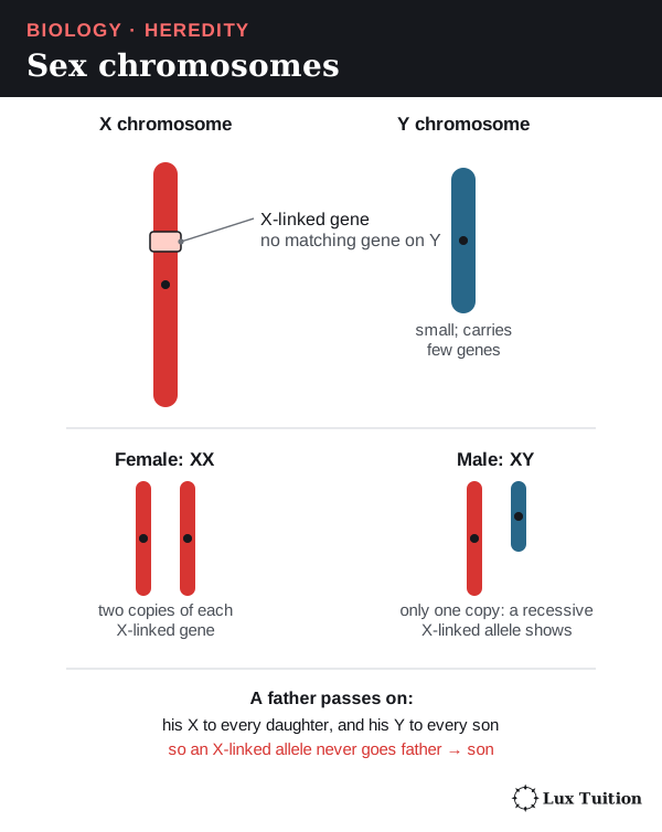
Humans have two sex chromosomes, X and Y; the others are autosomes. A sex-linked gene is on a sex chromosome; an autosomal gene is on an autosome.
- An XY person has only one copy of most X-linked genes, so a recessive X-linked allele shows its effect.
- A father passes his X to daughters and his Y to sons, so an X-linked allele never passes father to son.
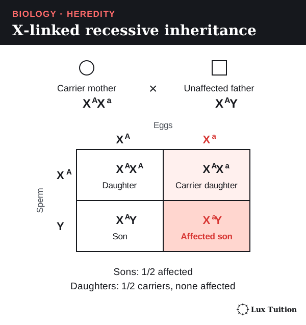
Worked example (X-linked recessive). Carrier mother (heterozygous, not affected) XAXa × unaffected father XAY: daughters are 1/2 XAXA and 1/2 XAXa (carriers, none affected); sons are 1/2 XAY and 1/2 XaY (affected). So half the sons are affected.
Assuming a son and a daughter are equally likely (1/2 each), any one child has a 1/2 × 1/2 = 1/4 chance of being an affected son.
Carrier females can sometimes show effects through X inactivation (one X switched off in each cell), so the simple model has limits.
For a fully penetrant (always expressed) X-linked dominant allele, an affected father and an unaffected mother have all daughters affected and all sons unaffected (sons get his Y, not his X).
An affected heterozygous mother can pass the allele to children of either sex, each with a 1/2 chance. Other organisms differ: in birds, females are ZW and males ZZ.
Linked genes
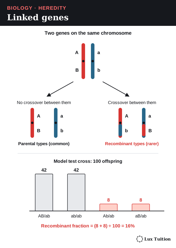
Linked genes are on the same chromosome, so they are inherited together more often than independent assortment predicts, unless crossing over separates them.
In a test cross AB/ab × ab/ab (one chromosome carries A and B, its partner a and b), 100 model offspring might be 42 AB/ab, 42 ab/ab and 8 Ab/ab, 8 aB/ab (recombinants). The recombinant fraction is (8 + 8) ÷ 100 = 16%.
- Below 50% supports linkage; 50% cannot separate unlinked genes from genes far apart on one chromosome.
- Double crossovers can hide some recombination.
How do you interpret pedigrees and inheritance patterns?
constructing and interpreting information and data from pedigrees and Punnett squares
A pedigree is a family-tree diagram showing how a phenotype appears across generations. Squares are males, circles females, and shading shows the phenotype (check the key), not the genotype. A horizontal line joins parents; a vertical line drops to their children. Generations are numbered I, II, III and individuals 1, 2, 3 from the left.
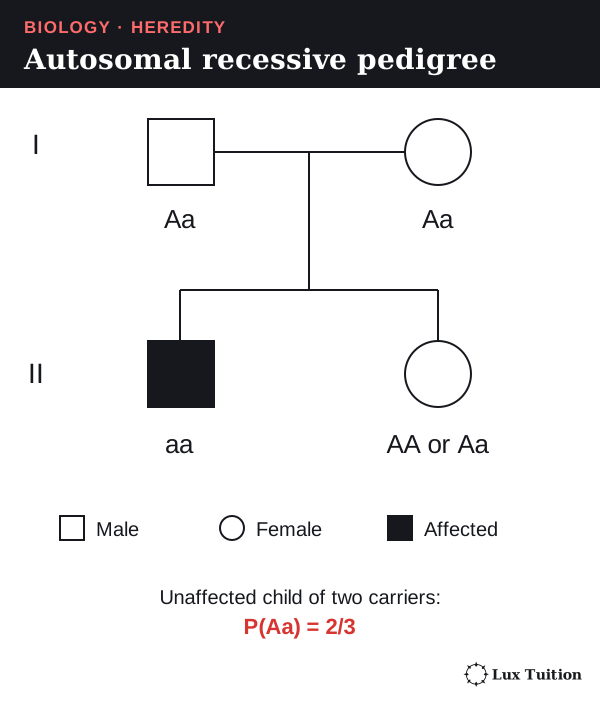
The table assumes a fully penetrant model (the allele always shows its effect).
| What you see | What it suggests | Important limit |
|---|---|---|
| Two unaffected parents have an affected child | Recessive inheritance; both parents can carry a recessive autosomal allele | A new mutation, incomplete penetrance or a wrong phenotype record could change this. |
| An affected father passes the trait to a son | Not consistent with direct X-linked inheritance | The son could have inherited an X-linked allele from his mother instead. |
| Both sexes are affected | Consistent with autosomal inheritance | It does not rule out X-linked inheritance. |
| The trait appears in every generation | Consistent with dominant inheritance | Recessive traits can also appear in successive generations. |
| All affected individuals are male | Can suggest X-linked recessive inheritance | A small family might show this pattern by chance with an autosomal gene. |
Worked example. Under an autosomal recessive model, unaffected parents of an affected (aa) child must both be Aa. Another child has chances 1/4 AA, 1/2 Aa, 1/4 aa. If that child is unaffected, aa is ruled out, leaving three equally likely outcomes (one AA, two Aa), so two of the three are Aa and the chance they are a carrier is 2/3.
A good answer assigns every possible genotype, checks every relationship for contradictions and states its assumptions. Small pedigrees can fit several modes of inheritance, and real family data needs consent and privacy.
How are allele and phenotype frequencies calculated?
examining frequency data
A population’s gene pool is all its alleles. Phenotype frequency is the fraction of individuals showing a characteristic; genotype frequency the fraction with a particular allele combination; allele frequency the fraction of all gene copies that are one allele.
Worked example. 100 diploid organisms: 20 AA, 30 Aa, 50 aa.
- There are 200 gene copies (two per organism).
- Copies of A = (2 × 20) + 30 = 70, so f(A) = 70/200 = 0.35.
- Copies of a = (2 × 50) + 30 = 130, so f(a) = 130/200 = 0.65 (check: 0.35 + 0.65 = 1).
- Genotype frequencies are 0.20, 0.30 and 0.50.
- If A is completely dominant, the dominant phenotype frequency is (20 + 30)/100 = 0.50, which is neither an allele nor a heterozygote frequency.
| Quantity | Calculation for a diploid autosomal gene |
|---|---|
| Genotype frequency | Number with that genotype ÷ total individuals |
| Allele A frequency | (2 × number AA + number Aa) ÷ (2 × total individuals) |
| Phenotype frequency | Number showing that phenotype ÷ total individuals |
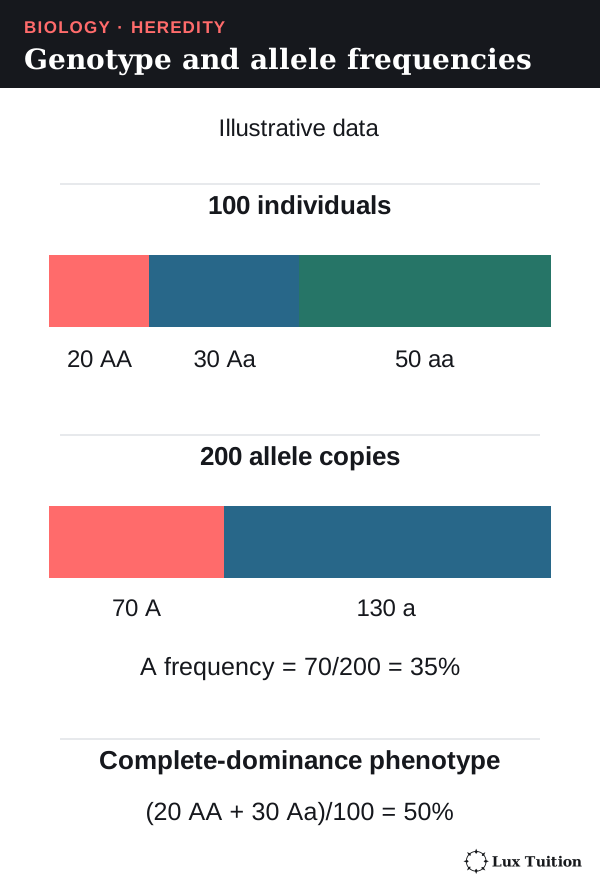
If a later, comparable sample has f(A) = 0.45, the frequency rose by 0.10 (ten percentage points), but that does not prove natural selection: migration, chance (genetic drift), mutation and sampling variation also contribute.
Samples must be comparable in place, age, method and size. Sampling relatives or one easy location can bias results (push them one way); bigger samples reduce random error but not bias.
Genetic drift and gene flow
Genetic drift is a change in allele frequencies caused by chance: which individuals happen to survive and reproduce, not which are best suited. It is stronger in small populations, because each individual carries a large share of the gene pool, so chance differences in who reproduces shift the frequencies a lot. In large populations, chance effects mostly cancel out.
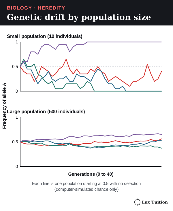
Gene flow is the movement of alleles between populations, when individuals (or their gametes, such as pollen) move and breed. It usually increases genetic diversity, but how much depends on population size:
- In a small population, one new allele is a big share of the gene pool, so diversity changes quickly. The new allele can spread fast if it is favoured, or be lost fast by drift.
- In a large population, one new allele is a tiny share, so frequencies change little.
So whether gene flow helps a population depends on its size and its environment: new alleles can add useful variation, or bring in alleles that are poorly suited to local conditions.
Use bar charts for categories and histograms for continuous measurements such as height, with units, consistent scales and clear totals. Compare frequencies when sample sizes differ, because counts alone can mislead.
What can SNPs and haplotypes reveal about genetic variation?
analysing single nucleotide polymorphism (SNP)
A single nucleotide polymorphism (SNP, “snip”) is a position where a single base varies between individuals. When the same stretch of DNA is lined up (aligned) from many people, some copies may have A and others G there; a person can then be AA, AG or GG, and allele frequencies are calculated as above.
- A SNP in a coding region (an exon read into amino acids) can change a protein. A SNP in a non-coding region (an intron, an untranslated region, or DNA between genes, which is never read into amino acids) usually leaves the protein unchanged, which explains a phenotype-neutral variant, although some non-coding SNPs affect regulation (how much a gene is switched on).
- A SNP linked to a phenotype may just be a marker near the real cause: association does not establish causation.
- A haplotype is a set of variants inherited together on one chromosome segment, so nearby SNPs are not necessarily independent evidence.
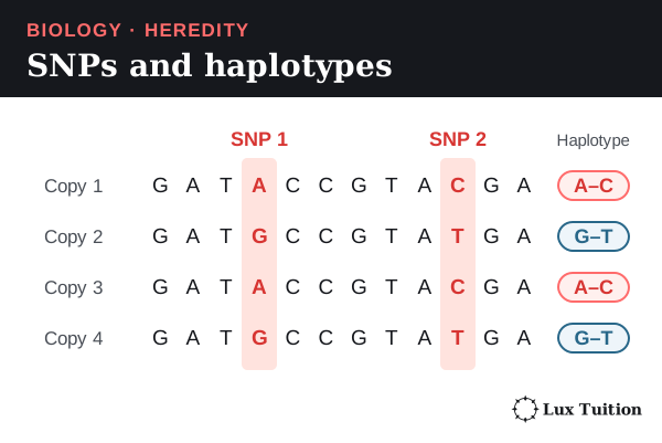
Comparisons need matching (homologous) regions, correct alignment and good-quality sequence, and one marker does not represent a whole genome. More matching positions generally support closer similarity for the sampled regions. Mutation rates vary between regions, recombination and gene flow shape the patterns, and databases can miss variation. Mitochondrial DNA (mtDNA) usually comes only from the mother, so it traces one line of ancestry; nuclear markers sample both parents’ lines.
Can population genetic patterns be predicted with any accuracy?
How do PCR, DNA sequencing and DNA profiling differ?
DNA sequencing and profiling (ACSBL086)
PCR makes many copies of a chosen piece of DNA; sequencing finds the order of its bases; profiling compares a few highly variable regions between people.
PCR (polymerase chain reaction)
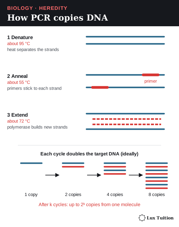
PCR needs primers: short single-stranded DNA pieces matching the two ends of the target. Each cycle:
- Denature: heat separates the strands.
- Anneal: cooling lets the primers bind on either side of the target, on opposite strands.
- Extend: a heat-stable DNA polymerase extends the primers into new strands using free DNA nucleotides.
Ideally the target doubles each cycle (2k copies after k cycles from one molecule). In practice efficiency falls and contaminating DNA can be copied too, so primer specificity and controls (comparison samples) matter.
Gel electrophoresis
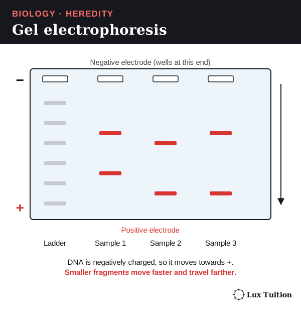
Electrophoresis separates DNA fragments by size. DNA is negatively charged, so it moves towards the positive electrode, and smaller fragments travel farther through the gel. A ladder of known sizes runs alongside. In capillary electrophoresis a detector shows each fragment as a peak: position gives size, while height shows signal strength rather than naming an allele.
DNA sequencing
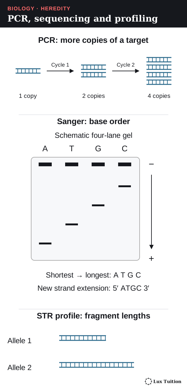
In Sanger sequencing, a primer is extended with normal nucleotides plus a few labelled chain-terminating nucleotides, which lack the 3′ hydroxyl (–OH) group, the chemical hook on the sugar that the next nucleotide must bond to, to add the next base. This makes fragments of every length, each ending in a labelled base. Sorted by size, shortest to longest, the labels spell out the new strand, which is complementary to the template.
High-throughput methods read many sequences at once and align them to a reference or assemble them by computer; quality and coverage (how often each base is read) affect confidence. See the NHGRI sequencing overview.
DNA profiling
Short tandem repeats (STRs) are short sequences repeated many times in a row. People differ in repeat number, so the copied region differs in length. A DNA profile compares lengths at several STR loci.
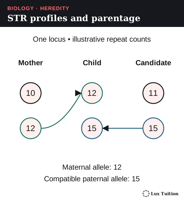
Worked example. A child gets one allele from each parent at an autosomal STR locus. Mother 10/12, child 12/15: assuming correct typing and no mutation, 15 came from the father. A candidate with 11/15 is compatible here, but one locus cannot prove parentage; many independent loci plus statistical evaluation are needed.
A profile match is not proof of guilt and cannot show how DNA got somewhere. Relatives share more alleles, identical twins normally share profiles, and contamination, damaged DNA or mixtures complicate interpretation (see the NIST DNA-mixture explainer).
How can population genetics guide koala conservation?
the use of population genetics data in conservation management
A large-scale collaborative project pools samples, lab work and analysis from many organisations. Conservation management is action to protect a species, such as moving animals between populations (translocation).
A 2016 koala study by Neaves and colleagues combined present-day and historical samples (from wildlife hospitals and museums) and compared one mitochondrial DNA control region. The present-day sample contained 662 koalas and 36 haplotypes, and their distribution revealed population structure (how genetically separate groups are).
- Koalas at Eyre Peninsula, Kangaroo Island and Bessiebelle had haplotypes similar to French Island koalas, fitting the recorded use of island koalas for translocations.
- Mt Lofty had comparatively high diversity among southern populations, fitting founders from a wider area, including NSW and Queensland.
So founding history shapes maternal diversity: populations far apart on a map need not have separate ancestry. Managers should check a population’s origin and remaining diversity before treating it as genetically distinct. Neaves et al., Discussion.
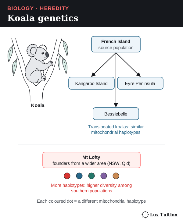
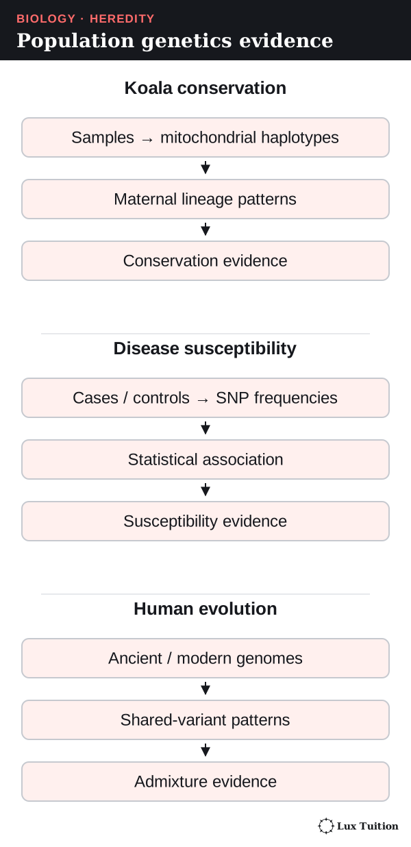
The reasoning chain: samples → sequences → haplotypes → their frequencies and locations → decisions about which populations join programs. Limits: mtDNA traces only the maternal line, sampling was uneven, few mitochondrial haplotypes does not mean identical nuclear genes, and translocation also needs ecological evidence and additional genetic evidence. Genetics supports, but does not replace, monitoring habitat, disease and numbers.
How do collaborative genetic studies identify disease susceptibility?
population genetics studies used to determine the inheritance of a disease or disorder
A case–control study compares people with a disease (cases) and without it (controls). If a SNP allele is more common in cases, the SNP is associated with the disease.
The Wellcome Trust Case Control Consortium’s 2007 study compared about 14,000 cases across seven common diseases with 3,000 shared controls at hundreds of thousands of SNPs, a scale that finds associations small family studies miss.
- It found 24 independent association signals at P < 5 × 10⁻⁷, including nine for Crohn’s disease (a bowel disease). P is the probability of getting results at least this extreme if there were no real association; a tiny P is strong evidence against “no association” but does not show the size or cause of an effect.
- Some regions were linked to more than one disease, hinting at shared biology.
- Many associated regions point to many genes contributing, not one allele that always causes disease.
These are statistical signals, not proof that each SNP causes disease. WTCCC 2007, abstract.
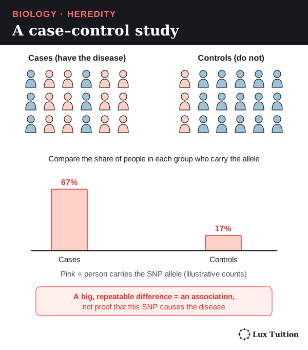
The analysis compares allele frequencies between groups, checks data quality, tests each difference statistically, and treats hits as starting points for finding mechanisms.
Limits: not everyone with a marker gets the disease; the typed SNP may not be causal; linkage, ancestry differences and the huge number of tests need care; replication in independent samples and functional evidence strengthen conclusions, and susceptibility depends on biological and environmental context; and a mostly European-ancestry sample limits generalisation. A susceptibility factor changes probability; it is not a diagnosis.
What can population genetics reveal about human evolution?
population genetics relating to human evolution
Neanderthals were an extinct group of humans in Europe and western Asia. The international 2010 Neanderthal draft-genome project compared ancient Neanderthal DNA with modern genomes and found evidence that Neanderthals interbred with ancestors of some present-day populations.
It used patterns of shared variants across the genome, not one matching base.
Genomes of people from Europe and Asia shared slightly more variants with Neanderthals than genomes from sub-Saharan Africa, suggesting the interbreeding happened after modern humans left Africa.
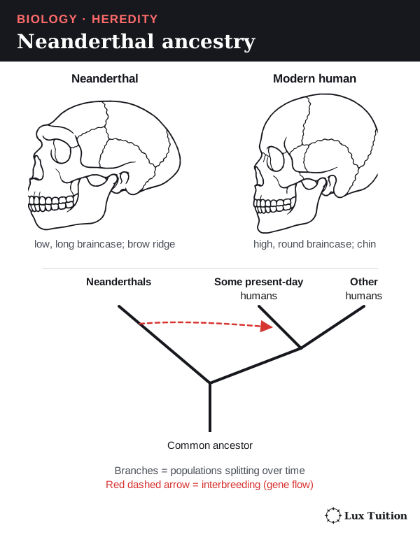
Limits: ancient DNA is fragmented and damaged; modern contamination can fake similarity, so results need authentication, suitable reference comparisons and statistical models; admixture (interbreeding between branches) adds links to a simple branching tree; estimates change with new samples and models; and mtDNA traces only the maternal line. Genetic patterns do not divide humanity into fixed, uniform categories.
Models and evidence in heredity
A model is a simplified representation, such as pipe-cleaner chromosomes or a paper DNA ladder. A chromosome model must keep homologous pairs, gene positions and sister chromatids consistent; a DNA model must keep complementary pairing and antiparallel strands; a translation model must keep template DNA, coding DNA, codons and anticodons distinct. State what the model leaves out (size, movement, chemistry, probability).
In model inheritance investigations, predicted ratios describe many chance events, so small samples vary. Record genotype counts before combining them into phenotypes, and pool independent results only from the same model and procedure, which can then improve precision. A mutation model changes a sequence; a crossover model swaps matching sections; they are different sources of variation.
Microscope evidence: the mitotic index
The mitotic index is the proportion of cells in mitosis: dividing cells ÷ total cells counted. For example, 24 ÷ 120 = 0.20, or 20%.
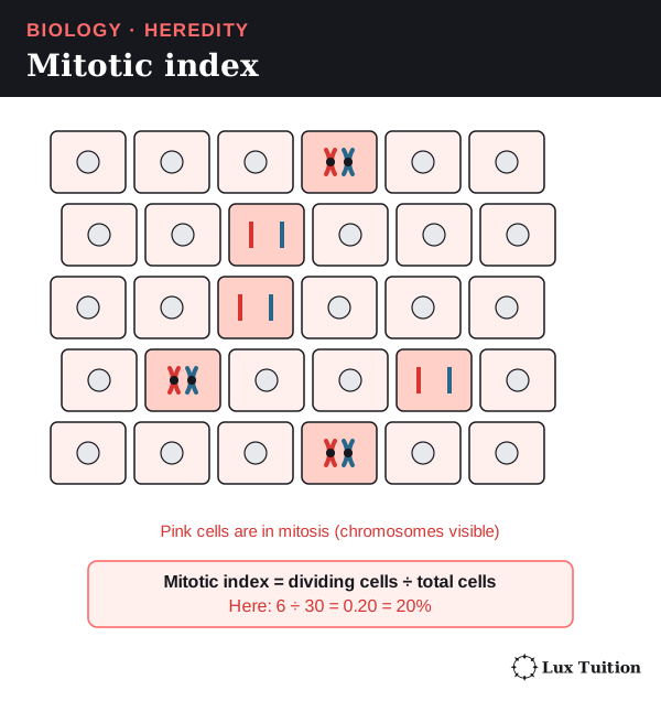
Using this snapshot to estimate time spent in a stage assumes cells divide at random times and the sample is representative; counting only the most active-looking region changes what the number describes.
These examples connect to the Working Scientifically skills below. Reading about investigations does not replace conducting and evaluating them.
Working Scientifically skills for Module 5
These are the investigation and data skills that HSC questions on heredity reward, taught with Module 5 examples.
Questions and hypotheses
A hypothesis is a proposed explanation that can be tested; a prediction says what you should observe if it is right. A testable hypothesis names what you change and what you measure, states the conditions, and could be shown wrong. A directional or comparative statement counts; adding a “because…” reason is a good habit, not a requirement.
When results do not fit: (1) name the result that does not fit, (2) check for a method problem, (3) rewrite the hypothesis to fit all the evidence, (4) test the new version with new data.
Module 5 example (based on 2020 HSC Q25). Hypothesis: “Animals using external fertilisation produce more eggs or young per reproductive cycle than animals using internal fertilisation.” Secondary data for six species of each kind gave means of about 40 ± 32 (external) and 43 ± 55 (internal), where ± means plus or minus. These values are written as mean ± standard deviation: 32 and 55 describe the spread within the two groups.
The means are similar and the spread within each group is far larger than the difference between them, so the data do not support the hypothesis.
A sensible revision narrows it (“within bony fish, external fertilisers lay more eggs”) and tests it on a larger, matched sample.
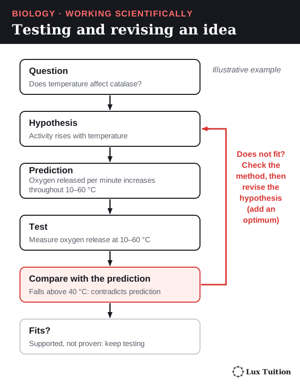
Common mistake: concluding “the hypothesis is proven” from data that only fit it. Data can support a hypothesis, never prove it.
Variables, controls and planning
The independent variable (IV), dependent variable (DV) and controlled variables are defined in the fungi section. An experimental control is an extra group or check that shows what happens without the factor being tested. The yeast counting-chamber investigation in the fungi section shows all three; here are two more Module 5 cases.
- A test with a built-in control (2021 HSC Q23). An LH ovulation test strip has a control line that should always appear, plus a test line that appears only if LH (luteinising hormone) is high. A strip showing the control line but no test line is a valid negative: the strip worked, and LH is not high. A strip with no control line is invalid whatever the test line shows.
- PCR controls. A negative control (all reagents but no DNA) should give no product; a band there means contamination. A positive control (DNA known to contain the target) should give a product, showing the reaction worked.
Replication. Use several independent samples per condition, as in the yeast example.
Planning: risk, ethics and materials. Write risks as hazard → harm → precaution: “Hot water bath for PCR heating (hazard) → scalds (harm) → use heat-proof gloves and let tubes cool (precaution).”
Ethics matters too: pedigree and DNA-profile data concern whole families, so they need consent and privacy, and animal breeding studies need ethics approval and minimal harm. Justify equipment: “A micropipette was used because it measures 10 µL accurately; a measuring cylinder cannot.”
Evaluating and modifying a plan. Tie each change to evidence: “The pilot culture at 35 °C overgrew the counting chamber, so samples were diluted 1 in 10 before counting.”
Accuracy, precision, validity and reliability
- Validity: the investigation answers the question it claims to. In a controlled experiment that means only the IV changes and the DV measures the right thing; an observational study is valid when exposure and outcomes are measured accurately and groups are matched or adjusted for confounders (other differences that also affect the outcome). Measuring CO₂ to show yeast reproduction is not valid, because CO₂ measures respiration, not cell number.
- Reliability: repeating it gives consistent results (independent replicate cultures give similar counts).
- Accuracy: closeness to the true value. A calibrated micropipette (checked against a known standard, such as weighing the water it delivers) gives accurate volumes.
- Precision: closeness of repeated measurements to each other. Resolution, the smallest change an instrument can show, limits precision.
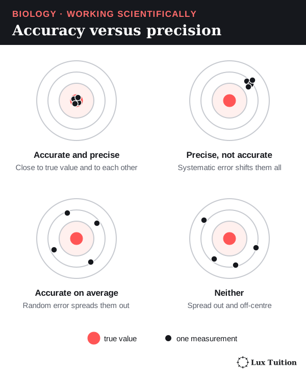
Random error scatters readings both ways (cells unevenly spread in the chamber); more replicates reduce its effect.
Systematic error shifts every reading by a fixed offset or proportion (always counting cells on all four edges of a square); averaging repeats cannot remove it, only a better method or calibration can.
Uncertainty is the range the true value probably lies in, and spread (range or standard deviation) shows how much results vary. Compare the spread within groups with the difference between groups, as in the fertilisation data above; overlapping ranges alone do not settle it, because sample size and the uncertainty in each mean also matter. Natural variation between organisms is not poor reliability.
To evaluate: name a specific limitation, say which quality it affects, and give a matching fix.
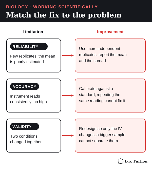
Common mistake: assuming repeats fix bias. Averaging independent readings reduces random uncertainty, but only calibration or a corrected method removes systematic bias.
Representing data
A categorical variable sorts data into groups (blood group, genotype); a continuous variable can take any value in a range (time, temperature).
- Bar or column graph: categories, such as the number of offspring of each phenotype from a cross.
- Histogram: how often values of one continuous measurement fall in each class (human height). Bars touch.
- Line graph: change over time (joining successive observations is fine for a recorded series), such as hormone levels across pregnancy or bacterial numbers during binary fission.
- Scatter graph: two measured continuous variables, with a line of best fit.
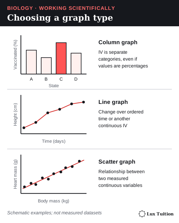
To draw a graph: IV on the x-axis, DV on the y-axis; label each axis with quantity and unit (“Time (h)”); choose an even scale that fills the grid; plot points as small crosses; use a key for more than one series.
Bacteria dividing by binary fission double every generation, so a graph of number against time curves steeply upwards (exponential growth, as in 2023 HSC Q5): do not force a straight line through it.
A line of best fit follows the trend with points balanced either side; when you draw one to show a relationship or predict, do not join the dots. Interpolation reads a value inside the measured range; extrapolation extends the trend beyond it, which assumes the trend continues.
Worked example (illustrative). The frequency of an allele R in a population is 0.11, 0.15, 0.23, 0.27 and 0.35 at generations 0, 2, 4, 6 and 8. When will it reach 0.5?
- Draw the line of best fit: it rises about 0.03 per generation.
- Extend it as a dashed line.
- Draw a construction line across from 0.5, then down to the x-axis: about generation 13.
- State the assumption: selection and other conditions stay the same.
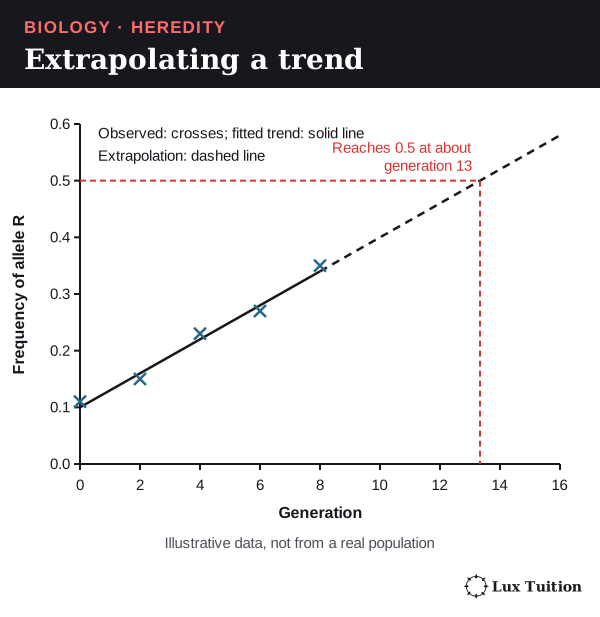
Quantitative methods
- Mean, median, range: for litter sizes 1, 6, 6, 18 the mean is 31 ÷ 4 = 7.75, the median is (6 + 6) ÷ 2 = 6 and the range is 17. One large value pulls the mean up, so report spread too.
- Expected counts from ratios: a 3 : 1 ratio among 400 offspring predicts 300 : 100. Real counts vary by chance, especially in small samples.
- Percentage change versus percentage points: f(A) rising from 0.35 to 0.45 is a rise of 10 percentage points, but a relative increase of (0.45 − 0.35) ÷ 0.35 × 100 ≈ 29%.
- Rate per 100,000: 30 babies born with a condition among 150,000 births is 30 ÷ 150,000 × 100,000 = 20 per 100,000.
- Converting a percentage to a count: if 4% of 5,000 people are carriers, 0.04 × 5,000 = 200 carriers.
- A population model (illustrative): if the frequency of allele a is q = 0.1 and mating is random, the model predicts q² = 0.01 (1%) of people are aa and 2 × 0.9 × 0.1 = 0.18 (18%) are carriers. This is a prediction from assumptions (random mating, no selection, migration or drift), not a measurement. Allele frequencies themselves are calculated as in the frequency section.
Models, trends and causes
A Punnett square predicts probabilities, not the actual order of births. PCR can be modelled as copies = 2k after k cycles; to reach about a million copies from one molecule, 220 ≈ 1,000,000, so about 20 cycles, assuming perfect doubling. Evaluate a model by stating what it explains, its assumptions and where those fail (real PCR efficiency falls in later cycles).
An association (two things changing together) is not proof of cause: see case–control studies and the SNP marker idea above. Describe a trend with values and units; explain it using established biology when the evidence supports that, and otherwise state what the data cannot establish; then evaluate how strongly the evidence supports it.
Secondary sources, arguments and communication
A secondary source reports data someone else collected. Judge who wrote it, where it was published (peer-reviewed journals and government agencies check work first), when, what evidence it shows and why it was written. Corroboration means independent studies with their own data agree.
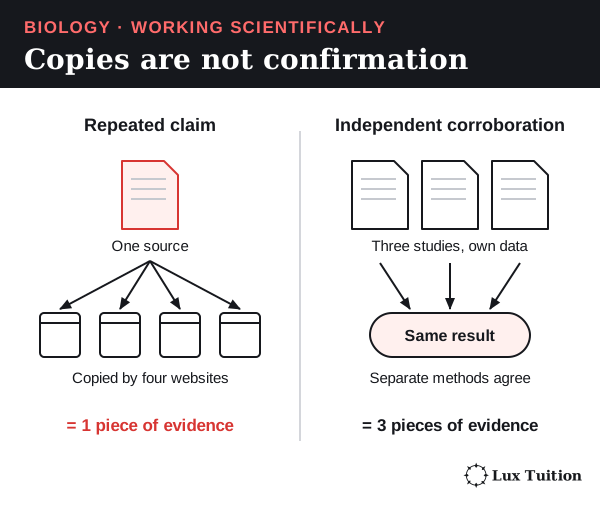
Check whether a sample represents the population: six species of each fertilisation type (2020 HSC Q25) cannot represent all animals, so a better study samples many species across groups. Reference each source consistently (author, year, title, publisher, URL and access date).
Build arguments as claim → evidence → reasoning → limitation. “This candidate cannot be excluded as the father (claim): he shares allele 15 with the child at the STR locus (evidence), and a child inherits one allele from each parent (reasoning). One locus cannot prove parentage (limitation).”
Answer criticism with evidence: when critics argued that matching ancient DNA could be modern contamination, the Neanderthal team showed authentication evidence such as the damage patterns typical of ancient DNA.
Communicate with the right format and notation: flow charts for sequences (gene → mRNA → ribosome → polypeptide, as in 2022 HSC Q31), Punnett squares and keys for crosses, and correct allele notation (XAXa, IAi).
Command words
| Command word | What your answer must do | Module 5 example |
|---|---|---|
| Identify | Name it | Identify the stage where sister chromatids separate (anaphase). |
| Describe | Give features, with values | Describe hCG levels across pregnancy. |
| Explain | Cause → mechanism → consequence | Explain why contractions strengthen during labour (positive feedback). |
| Analyse | Break into parts; show trends and links | Analyse the pedigree to show how the trait is inherited. |
| Discuss | Considerations on more than one side | Discuss the benefits and risks of genetic testing. |
| Compare | Similarities and differences | Compare mitosis and meiosis. |
| Assess | Judge value or size, with reasons | Assess the impact of artificial insemination on genetic diversity. |
| Evaluate | Strengths, limitations, then a judgement | Evaluate the use of mitochondrial DNA to guide koala translocation. |
| Justify | Support a claim with evidence | Justify which LH test strip is a valid negative. |
These shapes are guides, not formulas: what you need depends on the question and the evidence. Analyse needs evidence for each part; discuss needs a conclusion after the considerations. See the NESA glossary. Common mistake: describing when asked to explain, or giving no final judgement in “assess” and “evaluate”.
Where do these ideas connect across Year 12 Biology?
For mutation and the use of genetic technologies, continue to Module 6: Genetic Change. The other Year 12 notes are:
- Module 6: Genetic Change
- Module 7: Infectious Disease
- Module 8: Non-infectious Disease and Disorders
Return to the HSC Biology notes overview for course navigation and shared scientific skills.
Biology tutoring in Blacktown
Our Year 12 Biology classes in Blacktown connect the concepts with feedback on how students apply them. Classes have 1–5 students. See current pricing or enquire about a free trial.
Learn it properly with a specialist tutor at Blacktown or online across NSW. Enquire about a free trial — no cost, no obligation. See online formats and class sizes.
Realistic study tips to help you prepare better for assessments with less stress, plus a printable study planner